End Notes

To locate references such as “Cotra 2020,” consult the bibliography at the bottom of this page. You can quickly locate it by Ctrl+F for ‘bibliography’. (For references that are cited in the printed book rather than these online endnotes, see this bibliography instead).

A convenient alternative for accessing the bibliography is to download this library that can be used with the reference management software Zotero.

How to read this document:

• Endnotes are identified by a numbering scheme of the form “<chapter number>.<endnote number>”. For instance, endnote 42 to chapter 5 is (5.42). 
• Note that the numbering restarts with each chapter. For instance, there is an endnote number 2 in both chapters 1 and 2 – references in this document as (1.2) and (2.2), respectively.

Notes to the Introduction

(0.1) This thought experiment comes from Georgia Ray’s “The Funnel of Human Experience” (G. Ray 2018). A number of commentators have also pointed me to the popular short story “The Egg” by Andy Weir (2009), which has a similar premise.

(0.2) The idea of the “first human being” is a bit of poetic license: there is no strict dividing line between Homo sapiens and our forebears. Moreover, it’s not even clear that “we” should refer only to Homo sapiens: early humans mated with Neanderthals and Denisovans (L. Chen et al. 2020). These issues do not alter the upshot of this thought experiment.

While the timing of Homo sapiens’s speciation is sometimes cited as two hundred thousand years ago, expert consensus is now that it occurred three hundred thousand years ago (Galway- Witham and Stringer 2018; Hublin et al. 2017; Schlebusch et al. 2017; personal communication with Marlize Lombard, Chris Stringer, and Mattias Jakobsson, April 26, 2021).

(0.3) The best available estimate is 117 billion (Kaneda and Haub 2021).

(0.4) These and similar claims are based on combining estimates of the total human population (Kaneda and Haub 2021) and life expectancy at different times (Finch 2010; Galor and Moav 2005; H. Kaplan et al. 2000; Riley 2005; UN 2019c; WHO 2019, 2020). They should be treated as ballpark estimates.

(0.5) These numbers, which I’ve based on back-of-the-envelope calculations, are meant to be merely illustrative. The true figures, if we had them, would probably be slightly different from what I’ve used here. For more detail on the numbers given in the initial thought experiment (living through the life of every human being who has ever lived), see the report The scope of human experience, available on whatweowethefuture.com here. Another fun fact that didn’t make it into the book: You would have spent 6 days and 16 hours on the Moon.

(0.6) Slavery is absent today among what are (erroneously) known in the literature as socially “simple,” highly egalitarian hunter-gatherer societies, who are probably most similar to preagricultural human societies (Kelly 2013, Chapter 9). Slavery likely only became widespread after the emergence of sedentary societies following the agricultural revolution. Any estimate of the fraction of the population enslaved since then necessarily involves some guesswork. But the evidence that exists suggests that in many agricultural societies, around 10 to 20 percent of the population was enslaved. For example, in the second millennium AD, as much as one-third of the population of Korea was enslaved. A quarter to a third of the population of some areas of Thailand and Burma were enslaved in the seventeenth through the nineteenth centuries and in the late nineteenth and early twentieth centuries, respectively. The enslaved population of the city of Rome during the Roman Empire was estimated to be between 25 and 40 percent of the total population. Probably around a third of people in ancient Athens were enslaved. In 1790, approximately 18 percent of the American population was enslaved (Bradley 2011; Campbell 2004, 163; Campbell 2010; D. B. Davis 2006, 44; Hallet 2007; Hunt 2010; Joly 2007; Patterson 1982, Appendix C; J. P. Rodriguez 1999, 16–17; Steckel 2012). Slavery was abolished globally over the course of the nineteenth and twentieth centuries. 

Estimating the fraction of the population who owned enslaved people involves equal amounts of guesswork, but it is reasonable to think that the proportion of slaveholders was similar to the proportion of the enslaved. If one-quarter of the population in a society were enslaved, then one might reasonably guess that they were owned by the richest quarter of the society. For instance, in America in 1830, there were around two million enslaved people and, according to one survey, 224,000 slaveholders in the South. However, this assumes that only one person in a surveyed household should be considered a slave owner, but arguably we should count everyone in the whole household. Since the household likely would have included more than five people, this suggests that there were around two enslaved people per slave owner (R. Fry 2019; Lightner and Ragan 2005; O’Neill 2021b). And the US South probably had an historically high ratio of slave owners to enslaved people.

(0.7) I mean ‘most deadly’ measured by the total number of people killed. In per capita terms, several pre-industrial conflicts may have been even deadlier. On one popular estimate, Genghis Khan’s conquests account for the largest-ever relative death toll, killing more than 10% of the world population at the time, compared to 2.6% for World War II (White, 2011, 2012; available at Our World in Data, 2013). Other contenders for the war that caused the highest number of deaths relative to the world population at the time include the An Lushan rebellion (8th Century AD), and a series of violent conflicts AD 184–280 leading up to the ‘Three Kingdoms’ period, both in China (Cirillo & Taleb, 2016b, p. 31). It should be noted that both estimates of war deaths and of world population in pre-industrial times are highly uncertain (and in fact, estimates of the former are often based on crude estimates of the latter), so any estimate of per-capita war deaths for pre-industrial conflicts should be treated with caution. For an excellent discussion of trends in war prevalence and intensity, see Braumoeller (2019).

(0.8) In this thought experiment as I currently state it, you would live to the end of the lives of all those alive today, but not beyond. I am taking into account today’s greater life expectancy—if we only looked at the number of people, ignoring how long they live, then current people account for 7 percent of those who have ever lived (Kaneda and Haub 2021). If, for people currently alive, we only included their experience until the present moment— rather than until the expected end of their lives—their share of all experience would be closer to 6 percent, since many people have long lives ahead of them.

(0.9) One tenth of the current world population is roughly 775 million people. A population of that size for 1 million years amounts to 775 million millions, or 7.75×1014, life years. This is about 0.5% of the 3.7 trillion (or 3.7×1012) years lived so far. For the lifespan of mammalian species, see Barnosky et al. (2011, p. 53), Lawton & May (1995, p. 5), and Proença & Pereira (2013, p. 168).

(0.10) “Seconds” is about accurate if we maintain roughly the current population as long as Earth remains habitable. If we settle other solar systems or otherwise massively increase either the population or the life span of civilisation, then really it should be tiny fractions of seconds. It is not out of the question that the experience of all past and present people could correspond to a time interval that is shorter than the shortest one ever measured—2.47 zeptoseconds, or 2.47×10−19 seconds (Grundmann et al. 2020), many orders of magnitude less time than it would take for your eyes to chemically react to light before initiating a neural transmission (Weiner 2009). This would be the case if, for instance, for a hundred trillion years (until the end of the age of star formation) each of one hundred billion stars (the lower bound of typical estimates for the number of stars in our galaxy, the Milky Way) supported a population of ten billion people (approximately the current world population).

(0.11) Throughout this book, I drop the hyphen and use “longterm” as an adjective. I use “long term” as the noun phrase.

(0.12) See https://www.givingwhatwecan.org/.

Notes to Chapter 1

(1.1)  This example is modified from Reasons and Persons (Parfit 1984, 315).

(1.2) Though this is sometimes described as an ancient Chinese or ancient Greek proverb, its origin is unknown.

(1.3) Constitution of the Iroquois Nations 1910.

(1.4) Lyons 1980, 173.

(1.5) That said, some reciprocity-type reasons might motivate concern for future generations, too. We may not benefit from the actions of people in the future, but we benefit enormously from the actions of people in the past: we eat fruit from plants they bred over thousands of years; we rely on medical knowledge they developed over centuries; we live under legal systems shaped by countless reforms they fought for. Perhaps, then, this gives us reasons to “pay it forward” and do our part to benefit the generations to come.

(1.6) In the famous “to be, or not to be” soliloquy from Hamlet, “undiscovered country” refers to the afterlife: “But that the dread of something after death, / The undiscovered country from whose bourn / No traveller returns, puzzles the will / And makes us rather bear those ills we have / Than fly to others that we know not of?” In appropriating (and naturalising) that metaphor to refer instead to the future, I’m following the lead of the Klingon chancellor Gorkon from the eponymous Star Trek VI: The Undiscovered Country.

(1.7) Common estimates are 2.5 million (Strait 2013, 42) to 2.8 million years (DiMaggio et al. 2015).

(1.8) Özkan et al. 2002, 1797; Vigne 2011. If by ‘city’ we mean a permanent urban settlement of at least 10,000 people, then common estimates for when the first cities formed are 5,000 to 7,000 years ago. The Sumerian settlement of Uruk, in today’s Iraq, is often said to have surpassed the 10,000 population mark about 6,000 years ago (e.g. Banning, 1998, p. 196, Tab. 6.4; Garfinkle, 2013; Pollock, 2019) There are some other potential contenders for the world’s earliest city in today’s Ukraine and Pakistan (Feuerstein et al., 2008, p. 146; Müller et al., 2016, p. 347), albeit usually based on weaker evidence and lacking urban features such as complex hierarchy, professional classes, monumental public architecture and an administrative bureaucracy (Garfinkle, 2013).

(1.9) Barnosky et al. 2011, 3; Lawton and May 1995, 5; Ord 2020, 83–85; Proença and Pereira 2013, 168.

(1.10) I don’t mean to make any strong claim that no nonhuman animals possess any abstract reasoning or longterm planning abilities whatsoever, or that none of them use any tools. There is ample evidence for several species arguably planning hours or even days ahead (e.g., Clayton et al. 2003; W. A. Roberts 2012), and tool production and use in apes is well documented (Brauer and Call 2015; Mulcahy and Call 2006). More broadly, animal cognition is a topic of ongoing empirical research and lively philosophical debate (for an overview, see Andrews and Monsó 2021).

(1.11) Estimates of how long the sun will continue to burn range from 4.5 billion (Bertulani 2013) to 6.4 billion years (Sackmann et al. 1993), though 5 billion seems to be the most common rough figure. More precisely, this refers to the time by which all hydrogen in the sun’s core will be used up, at which point the sun will begin to leave what astronomers call the “main sequence” of stars. However, it is still going to “burn”—that is, to generate energy through nuclear fusion of hydrogen into helium, albeit in its shell rather than its core. After it expands as a red giant for about two to three billion years, nuclear fusion is going to resume in the core—this time fusing helium into carbon and oxygen—and only after this final helium flash will the sun stop shining altogether, about eight billion years into the future.

The figure for conventional star formations is from F. C. Adams and Laughlin 1997, 342.

I am grateful to Toby Ord for making me aware of how long a few stars will continue to shine. Anders Sandberg, in his upcoming book Grand Futures, notes that on even longer timescales, after the end of those stars, there are more exotic sources of energy, such as black holes, which could be harnessed. This could extend civilisation’s life span beyond a million trillion years.

(1.12) Wolf and Toon (2015, 5792) estimate that “physiological constraints on the human body imply that Earth will become uninhabitable for humans in ~1.3 Gyr [1.3 billion years]”; Bloh (2008, 597) gives a somewhat shorter window, stating that the “life spans of complex multicellular life and of eukaryotes end at about 0.8 Gyr and 1.3 Gyr from present, respectively.” I am going with a more conservative window of human habitability of perhaps five hundred million years because of considerable uncertainty about the timing and likelihood of key developments—such as plants dying from carbon dioxide starvation, or a “runaway greenhouse effect” leading to the evaporation of the oceans—and the open question of which of these will be the limiting factor for human habitability (see Heath and Doyle [2009] for a survey of considerations that affect the habitability of planets for different types of life).

One plausible contender is C3 photosynthesis becoming impossible due to falling CO2 levels, which would cause most trees (Young et al., 2020) and many food crops to die out. This may or may not happen significantly earlier than 1 billion years from now: Lovelock & Whitfield (1982) gave a first estimate of 100 million years; using a more accurate climate model, Caldeira & Kasting (1992, p. 722) found a timeframe of 500 million years instead; taking into account yet another consideration — silicate rock weathering — Lenton & von Bloh (2001) conclude that temperature rather than CO2 levels may limit Earth’s habitability for plants after all, extending the deadline to 800 million years or more. The cause of all these developments is the Sun’s increasing brightness. The Earth’s window of habitability for all life is significantly longer, with O’Malley-James et al. (2013, p. 99) estimating that “unicellular life could persist for up to 2.8 Gyr from present” in certain niches such as mountains and caves. The Earth thus will become barren long before it will be swallowed by the Sun in its expanding ‘red giant’ stage, which is projected to happen in about 7.5 billion years (Schroder & Connon Smith, 2008), contrary to some earlier estimates that had left open whether the Earth might narrowly escape that fate. One caveat to all these numbers is that, over these enormous time scales, technological progress or even evolutionary adaptation might dramatically alter the range of conditions in which humanity’s descendants can survive.

(1.13) Global population density, if we exclude water and Antarctica, is about 57 people per km2. The World Bank gives the Netherlands’ population density (in 2020) as 518 people per km2 (World Bank, 2021), about 9 times larger. So if the world’s land mass, excluding Antarctica, was as densely packed with people as the Netherlands, its population would be about 9 times larger than the current 7.75 billion, or about 70 billion.

(1.14) There are one hundred to four hundred billion stars in our galaxy, the Milky Way. The number of reachable galaxies has been estimated as 4.3 billion by Armstrong and Sandberg (2013, 9) while Ord (2021, 27) states, “The affectable universe contains about 20 billion galaxies with a total of between 1021 and 1023 stars (whose average mass is half that of the Sun).”

(1.15) My figures are for life expectancy at birth (Roser 2018). Since, in the early nineteenth century, about 43 percent of children globally died before age five (Roser 2019), someone surviving until that age could expect to become about fifty years old. Note also that seventy-three years is not necessarily the best prediction for how long someone born today is going to live: the figures I quoted are for what’s known as “period life expectancy,” a measure of life expectancy that by definition ignores future trends. For instance, if there will be further progress in medicine and public health, then someone born today should in fact expect to live longer than seventy-three years; on the other hand, if new deadly diseases will emerge or a large fraction of the world population will be wiped out by a large-scale catastrophe, someone born today should expect to live a shorter life than suggested by their period life expectancy at birth.

(1.16) In 1820, an estimated 83.9 percent of the world population lived on a daily income that, adjusted for inflation and price differences between countries, bought less than one dollar did in the US in 1985 (Bourguignon and Morrisson 2002, Table 1, 731, 733). In 2002, when Bourguignon and Morrisson published their seminal paper on the history of the world income distribution, this was the World Bank’s international poverty line, typically used to define extreme poverty. The World Bank has since updated the international poverty line to a daily income corresponding to what $1.90 would have bought in the US in 2011. Using this new definition, World Bank data indicates that the share of the global population living in extreme poverty has been less than 10 percent since 2016; the COVID-19 pandemic tragically broke the long-standing trend of that percentage declining year after year, but it did not quite push it over 10 percent again (World Bank 2020). While the extent to which the old and new poverty lines match is often debated, I think the conclusion that the share of the world population in extreme poverty declined dramatically is unambiguous. This is not to deny we still have a long way to go in the fight against poverty; for instance, more than 40 percent of the world population still live on less than $5.50 per day (again, adjusted for inflation and international price differences relative to the US in 2011).

(1.17) Roser and Ortiz-Ospina 2016.

(1.18) Our World in Data 2017a. Our well-off Brit may also have lost up to two-thirds of his children: “Infant and child mortality more than doubled between the sixteenth and the middle of the eighteenth century in both wealthy and non-wealthy families […]. Mortality peaked in the middle of the eighteenth century at a very high  level, with nearly two-thirds of all children — rich and poor — dying by their fifth birthday.” (Razzell & Spence, 2007, p. 271)

(1.19) There are a few rumoured cases of women being awarded degrees or teaching at universities prior to 1700, but their lives are usually poorly documented. Bettisia Gozzadini may have delivered lectures in law at the University of Bologna in the 13th century, and may be the first woman to have ever taught at a university (Eco, n.d.), though this is disputed (Morata, 2003, p. 30). The handful of other potential cases preceding the 17th century are clouded in similar uncertainty. For a more definite case we have to wait until 1678, when Elena Lucrezia Cornaro Piscopia obtained a Doctor of Philosophy from the University of Padua—the Encyclopedia Britannica maintains that Cornaro “was the first woman to receive a degree from a university”—and even she was barred from her preferred degree (theology) by the bishop of Padua (Gregersen, 2021). In any case, it seems clear that, in 1700—when there were at least several dozens of universities across Europe (Ridder-Symoens & Frijhoff, 1996, pp. 80–89)—, higher education was almost exclusively accessible to men; we remember and discuss potential exceptions precisely because they were very rare.

(1.20) “Throughout the eighteenth century and up until 1861, all penetrative homosexual acts committed by men were punishable by death” (Emsley et al. 2018).

(1.21) “At the end of the eighteenth century, well over three quarters of all people alive were in bondage of one kind or another, not the captivity of striped prison uniforms, but of various systems of slavery or serfdom” (Hochschild 2005, 2). The numbers for today—40.3 million, or about 0.5 percent of the world population—include both forced labour and forced marriage (Walk Free Foundation 2018).

(1.22) While the broad trend of increasing political liberties and individual autonomy strikes me as incontrovertible, the exact numbers depend on the definition of democracy. I got mine from Our World in Data’s page on “Democracy” (Roser 2013a), which is based on the widely used Polity IV data set. Its democracy score is a composite variable that captures different aspects of measuring “the presence of institutions and procedures through which citizens can express effective preferences about alternative policies and leaders” and “the existence of institutionalized constraints on the exercise of power by the executive” but excludes measures of civil liberties (Marshall et al. 2013, 14). My claim about the year 1700 is based on the assumption that the situation then can’t have been much better than in the early nineteenth century, when Polity IV has less than 1 percent of the world population living in a democracy. I’m also making the definitional judgment call to exclude societies without full-blown statehood (e.g., hunter-gatherers) even if some of them might have had protodemocratic features such as inclusive participation in deliberation or checks on leaders’ ability to abuse power.

(1.23) Gillingham 2014, Wyatt 2009. In total, the British Empire bought more than three million enslaved people during the transatlantic slave trade, and France bought more than one million (Slave Voyages 2018).

(1.24) Sonnets 1–126 are typically considered to be addressed to a “young man,” though, like many aspects of Shakespeare’s life and works, this remains a subject of scholarly debate. For instance, in the Introduction to the 2002 edition of Shakespeare’s Complete Sonnets and Poems, Burrow notes that “[m]any of the poems in the group 1–126 which since Malone have been treated as poems to a ‘young man’ carefully skirt around even giving a fixed gender to their addressee.” (Shakespeare, 2002). Erne (2007, p. 63) cites Leishman (1961, p. 22) stating that Shakespeare “has written both more copiously and more memorably on this topic [i.e. poetry as immortalization] than any other sonneteer.” Famous in this vein are also the opening verses of Sonnet 55: “Not marble, nor the gilded monuments / Of princes shall outlive this pow’rful rhyme,” (Shakespeare, 2002, p. 491).

(1.25) Shakespeare 2002, 417.

(1.26) Shakespeare “had likely drafted the majority of his sonnets in 1591–95” (Kennedy 2007, 24). Kennedy cites Hieatt et al. (1991, 98) who, based on an analysis of rare words appearing in Shakespeare’s works throughout his career, specifically suggest that “many of” Sonnets 1–60 were first drafted between 1591 and 1595.

(1.27) Horace published the first three books of his Odes in 23 BC (Grant, 2020). I am quoting from the final poem of book three. Another example comes from Ovid. As English literature Professor Jacob Sider Jost comments, in the Metamorphoses (written in AD 8) Ovid spends a full fifteen books emphasising how all things are in flux and change, then proclaims that his own poetry is the exception to the rule: “And now my work is done, which neither the wrath of Jove, nor fire, nor sword, nor the gnawing tooth of time shall ever be able to undo.… I shall have an undying name.” (Sider Jost, 2015).

(1.28) Horace 2004, 216–217.

(1.29) It is clear that Thucydides witnessed much of the war 431–404 BC, though his History “stops in the middle of the events of the autumn of 411 BC” (Gomme, 2020). In part for this reason, Gomme (2020) states that “time and manner of his [Thucydides’s] death are uncertain, but that he died shortly after 404 is probable”.

(1.30) For instance, Bury (1900/2015, p. 252) describes the History as “severe in its detachment, written from a purely intellectual point of view, unencumbered with platitudes and moral judgments, cold and critical.” Some more recent scholarship disputes this interpretation, instead characterizing Thucydides as “an artist who responds to, selects and skillfully arranges his material, and develops its symbolic and emotional potential.” (Connor, 1985, pp. 231–232).

(1.31) The quote is from Rex Warner’s 1954 translation as printed in the 1972 Penguin Books edition (Thucydides 1972). The same passage in the Charles Forster Smith translation from the Loeb Classical Library reads as follows: “[…] but whoever shall wish to have a clear view both of the events which have happened and of those which will some day, in all human probability, happen again in the same or a similar way—for these to adjudge my history profitable will be enough for me. And, indeed, it has been composed, not as a prize-essay to be heard for the moment, but as a possession for all time.” (Thucydides, ca. 425 B.C.E./1919, p. 41).

(1.32) Bornstein 2015, 661; Holmes and Maurer 2016.

(1.33) J. Adams 1851, 298. Incidentally, in the same preface, Adams quotes Thucydides at length, including part of the passage I referenced earlier.

(1.34) My rendition of how Franklin’s will came about employs some interpretative best guesses. What we know with certainty is that the French mathematician and essayist Charles Joseph Mathon de la Cour, in August 1784, published a piece titled Testament de M. Fortuné Ricard (de la Cour, 1784). The testament declares that 500 livres are to be invested with compound interests, and to be spent over the next 500 years for various social projects (one of my favorites is that, after 500 years, a part of the accumulated funds is to pay for all of France’s national debt, but only under the condition that “the Kings […] order the comptrollers general of the finances to undergo in future an examination in arithmetic before they enter upon their office” (de la Cour, 1785/2013)). Franklin served as US ambassador to France 1776–1785, and was well known among the French elite—the 11th edition of the Encyclopedia Britannica states that, when he arrived in Paris, Franklin was “one of the most talked about men in the world”, and quotes the historian Friedrich Christoph Schlosser as saying “[s]uch was the number of portraits, busts and medallions of him [Franklin] in circulation before he left Paris that he would have been recognized from them by any adult citizen in any part of the civilized world.” (R. Webster, 1911). Prior to his diplomatic service, Franklin had become wealthy and famous as a publisher, and among his most successful titles was the series Poor Richard’s Almanack, which he authored yearly for 25 years, starting in 1732, using the pseudonyms Richard Saunders or Poor Richard (R. Webster, 1911). The Almanacks “far exceed[ed] the sale of any other publication in the [American] colonies” (R. Webster, 1911). Mathon de la Cour appended his ‘Testament’ to a letter to Franklin from 30 June, 1785, in which he also expresses his admiration for Franklin: “During the last years of my residence at Paris, my heart often beat with joy when I had an opportunity of joining my applause to that which all France seemed to think due to you, wherever you appeared.” Considering this background, it seems highly likely that the ‘Testament of Fortunate Richard’ was conceived as a tribute to Franklin’s alter ego Poor Richard. We also know about Franklin’s reaction, who stated in a letter to Mathon de la Cour, dated Nov. 18, 1785, “The reading of Fortuné Ricard’s Testament has put it into the head and heart of a citizen to leave two thousand pounds sterling to two American cities […]” and continued to describe an arrangement very similar to the one he appended to his will in 1789 (Franklin, 1818, p. 203). For Franklin’s will, see Franklin (1904, pp. 200–223), with the bequest to Boston and Philadelphia being described within the ‘Codicil’ on pp. 213–219. An English translation of Fortuné Ricard’s Testament appeared in 1785 as an appendix to Richard Price’s Observations on the Importance of the American Revolution, with a note that the Testament was “conveyed to me by Dr. Franklin” (de la Cour, 1785/2013).

(1.35) Franklin’s bequest is well known. My source for the numbers given in the main text is the epilogue of Isaacson (2003, 473-474) Regarding the currency and inflation conversion, Isaacson (2003, Chapter 15) indicates that, in 1790, £1,000 were worth $4,520; and according to US inflation data, this corresponds to $135,889.38 in 2021 (I. Webster, 2021). (The equivalent sum in 1990, when Franklin’s trusts were paid out, is $64,213.48. So in inflation-adjusted terms, Franklin’s trust for Boston grew by a factor of 78 over 200 years, and the Philadelphia trust by a factor of 36.)

(1.36) “It can be said, as Adams did, that the declaration [of independence] contained nothing really novel in its political philosophy, which was derived from John Locke, Algernon Sidney, and other English theorists.” (Encyclopedia Britannica, 2021). “The French political theorist Montesquieu, through his masterpiece The Spirit of the Laws (1748), strongly influenced […] many of the American Founding Fathers, including John Adams, Jefferson, and Madison.” (Dahl, 2021). Regarding Polybius’s influence on Montesquieu, Edelstein (2019, p. 269) in a review of Benjamin Straumann’s book Crisis and Constitutionalism, writes that “Straumann argues, very cogently, that scholars have overlooked the influence of Polybius and Cicero on Montesquieu’s constitutionalism.” For Greco-Roman influences more broadly, see Gummere (1955).

(1.37) Lloyd 1998, Chapter 2.

(1.38) Lord et al. 2016; Talento and Ganopolski 2021. Of course, we might later remove carbon dioxide from the atmosphere. But we should not be very confident that we will do this, and certainly not in light of the possibilities of collapse and stagnation that I discuss in Chapters 6 and 7. I discuss the longtermist importance of burning fossil fuels in more detail in Chapter 6.

(1.39) Hamilton et al. 2012.

(1.40) The average life span of carbon dioxide shows another way in which current climate rhetoric and policy is shortsighted: the comparison with methane. Methane is often claimed to have thirty or even eighty-three times the warming potential of carbon dioxide, or even more. But from a longterm perspective, these numbers are misleading. Methane only stays in the atmosphere for about twelve years (IPCC 2021a, Chapter 7, Table 7.15); this is in stark contrast to carbon dioxide, which, as we’ve seen, stays in the atmosphere for hundreds of thousands of years.

The most commonly used weighting for methane has been to treat it as thirty times as important as carbon dioxide, but this metric measures the effect methane has on temperatures after forty years. (Confusingly, this metric is known as “Global Warming Potential.”) If instead we measure the effect that methane has on temperatures in one hundred years, methane is only 7.5 times as potent as carbon dioxide (IPCC 2021a, Chapter 7, Table 7.15).

Though the weight we give to methane rather than carbon dioxide is usually presented as a scientific matter, really it’s primarily about whether we wish to prioritise reducing climate change over the next few decades or over the long run (Allen 2015). Given that we emit sixty times as much carbon dioxide as methane, if we take a longterm perspective, it’s carbon dioxide that should be our main focus (H. Ritchie and Roser 2020a; Schiermeier 2020).

(1.41) P. U. Clark et al. 2016.

(1.42) IPCC 2021a, Figure SPM.8. The medium-low-emissions scenario is known as RCP4.5 (Hausfather and Peters 2020; Liu and Raftery 2021; Rogelj et al. 2016).

(1.43) Clark et al. (2016, Figure 4a) project that on a medium-low-emissions scenario, sea level would rise by twenty metres. Van Breedam et al. (2020, Table 1) find that sea level would rise by ten metres on the medium-low pathway.

(1.44) P. U. Clark et al. 2016, Figure 6.

(1.45) “Air pollution is associated with many health impacts, including chronic obstructive pulmonary disease (COPD) linked to enhanced ozone (O3), and acute lower respiratory illness (ALRI), cerebrovascular disease (CEV), ischaemic heart disease (IHD), COPD and lung cancer (LC) linked to PM2.5 [i.e., fine particulate matter with a diameter smaller than 2.5 micrometres]” (Lelieveld et al., 2015, p. 367). Fossil fuels are a main source of PM2.5 pollution (Lelieveld et al., 2019).

(1.46) Our World in Data 2020a, based on Lelieveld et al. 2019. This only includes deaths from outdoor air pollution. An additional 1.6 million (Stanaway et al. 2018) to 3.8 million (WHO 2021) excess deaths per year are due to indoor air pollution, much of which is caused by lack of access to electricity and clean fuels for cooking, heating, and lighting (H. Ritchie and Roser 2019). More than 2.5 billion people are able to cook only by burning coal, kerosene, charcoal, wood, dung, or crop waste using inefficient and unsafe technology such as open fires (WHO 2021).

(1.47) “In Europe an excess mortality rate of 434 000 (95% CI [confidence interval] 355 000–509 000) per year could be avoided by removing fossil fuel related emissions. . . . The increase in mean life expectancy in Europe would be 1.2 (95% CI [confidence interval] 1.0–1.4) years” (Lelieveld, Klingmüller, Pozzer, Pöschl, et al. 2019, 1595). A 95 percent confidence interval indicates the range in which, based on the authors’ model, the true number falls with a probability of 95 percent. Note that the authors use spacing rather than commas when formatting large numbers—e.g., “434 000” refers to four hundred thirty-four thousand.

(1.48) Scovronick et al. (2019, 1) found that depending on air-quality policies and “on how society values better health, economically optimal levels of mitigation may be consistent with a target of 2°C or lower.” Markandya et al. (2018, e126) found that the “health co- benefits substantially outweighed the policy cost of achieving the [2°C] target for all of the scenarios that we analysed” and that “the extra effort of trying to pursue the 1.5°C target instead of the 2°C target would generate a substantial net benefit in India (US$3.28–8.4 trillion) and China ($0.27–2.31 trillion), although this positive result was not seen in the other regions.”

(1.49) The claim that we live in a highly unusual period in history also raises some interesting philosophical issues, as I discuss in my article “Are We Living at the Hinge of History?” (for a draft see MacAskill 2020, formal publication forthcoming). However, note that the arguments in that article are against the idea that we’re at the most influential time ever. I think the case for thinking that we’re (“merely”) at an enormously influential time is very strong.

(1.50) This argument and framing follows Holden Karnofsky’s “This Can’t Go On” (2021b), which builds on an argument by Robin Hanson (2009). Mogensen (2020, sec. 5) points out one way in which some versions of longtermism would have arguably counterintuitive conclusions even if our time was less unusual. However, his discussion only applies to versions of longtermism on which our obligation to help future people trumps all other self- and other-regarding reasons for action, which is not the view I’m defending in this book. See also my discussion of longtermism versus ‘strong longtermism’ in this book’s Appendix.

(1.51) More precisely, I’m thinking of the present as a postindustrial era that began 250 years ago and will end whenever growth rates slow again to below 1 percent per year. For recent growth rates, see World Bank (2021e).

(1.52) For all claims about the history of global growth, see, for instance, DeLong (1998). For an overview of other data sources, which give similar numbers, see Roodman’s (2020a) data and Roser’s (2019) data sources. Note that my claims are about average growth rates that are being sustained for several doubling times—we cannot, of course, rule out that the growth rate may have been 2 percent in a single year in, say, 200,000 BC (but we know that, if this happened, it must have been an exception). For a discussion of intermittent brief periods of above-average growth in world history, see Goldstone (2002), though my background research for Chapter 7 suggests that some examples therein are controversial.

(1.53) Energy use: Our World in Data 2020f; carbon dioxide emissions: Ritchie and Roser 2020a; land use: Our World in Data 2019b. Measurements of scientific advancement are subject to interpretation, but I believe that few would disagree with the claim that the pace of technological innovation has rapidly accelerated since the Scientific Revolution in the sixteenth century compared to premodern times.

(1.54) This is in fact closer to what growth has been at the technological frontier—that is, ignoring the transient catch-up growth of poorer countries (Roser 2013b).

(1.55) Karnofsky 2021b, nn7–8.

(1.56) For further discussion about whether it’s possible, see Hanson 2009 and Karnofsky 2021c.

(1.57) I thank Carl Shulman for this point.

(1.58) Of course, many groups within a single continent may have never communicated as well. My figure of 50,000 years ago simply is an estimate of the time by which humans had dispersed out of Africa onto several other continents (Haber et al., 2019; Karmin et al., 2015; Posth et al., 2016; Rito et al., 2019). This is a rough upper bound for the time since which there must have been several largely isolated human populations, based on the assumptions that, given prehistoric technology, human populations cannot have communicated across continents except perhaps for some groups on either side of two continents’ shared border.

(1.59) Scheidel (2021, 101–107) provides a summary of historic empires’ population sizes; his Table 2.2 (103) indicates that the Western Han dynasty comprised 32 percent of the world’s population in AD 1, while in AD 150 30 percent lived in the Roman Empire. There is, however, considerable uncertainty about historic population sizes; The historian Peter Bang (2009, 120) has commented that even at their peak, the Han and the Roman Empires “remained hidden to each other in a twilight realm of fable and myth.” Other estimates are closer to 25 percent each for the Han dynasty (Sadao, 1986, p. 596) and Rome (Frier, 2000; Harper, 2018; Scheidel, 2007)—numbers converted to a percentage of world population using the absolute world population estimate from Maddison for AD 1 and HYDE 3.2 for AD 150 (Goldewijk et al., 2017; Maddison, 2010). 

(1.60) This treats the orbit of the outermost planet, Neptune, as the boundary of the solar system. The diameter of the Milky Way is 100,000–200,000 light years, or about 1021 m. The diameter of the Earth is about 1.3×107 m — smaller than the Milky Way by a factor of about 1014. Using a diameter of 60 AU – about 1013 m – for the solar system, and scaling it down by that factor, results in 10 cm. (If, instead of Neptune’s orbit, we used a different boundary for the solar system, that number would be larger: up to about 1 m if we used the Kuiper belt or the distance at which the Sun’s solar wind slows down to subsonic speed [‘Termination shock’] or stops [‘heliopause’]; and up to hundreds of meters, the same order of magnitude as the distance to Alpha Centauri, if we used the Oort cloud. Since in this context we are concerned with interstellar communication, and space settlements would most likely be located on planets with stable orbits around the Sun or their satellites – and possibly artificial structures closer to the Sun – the Neptune-based definition seems most appropriate to use.) The nearest star system is Alpha Centauri, about 4.4 light-years, or 4.1×1016 m, from the Sun—about 400 m on our scale.

(1.61) My estimate for the number of galaxy clusters is based on separate estimates for the numbers of galaxies and the number of galaxies per cluster, respectively. Since there is considerable uncertainty about both of these, the number of galaxy clusters might be, as far as I can tell, anywhere between ‘tens of thousands’ and ‘hundreds of millions’. Ord (2021, p. 39) gives a number of 20 billion galaxies in the affectable universe. This is less than 5% of the galaxies in the observable universe, but arguably the affectable universe is the best scope to consider in this context since we are concerned with a scenario in which humanity, starting from Earth, settles other galaxies. The Encyclopedia Britannica gives the number of galaxies per cluster as ranging “from the hundreds to the tens of thousands” (Encyclopedia Britannica, 2018) . This suggests there are between 200,000 and 200 million galaxy clusters in the observable universe. However, Ord’s number of galaxies is based on Conselice et al. (2016), which might be an overestimate (Lauer et al., 2021, p. 22) – for all I know this could cut the number of galaxy clusters by another factor of 10. My best guess is toward the higher end of the range because the lower estimates for the number of galaxies per cluster seem more common – e.g. the website of the Chandra X-ray observatory at Harvard just says “hundreds of galaxies” (NASA, 2012).

(1.62) Technically, the astronomical term of art for groups of galaxies that are ‘virialised,’ i.e. gravitationally bound and no longer collapsing or expanding, is galaxy cluster (e.g. Chon et al., 2015, p. 1), with ‘galaxy group’ sometimes referring to collections of galaxies defined by other means, usually smaller. Determining which currently observable collections of galaxies are going to form clusters in the future, rather than being torn apart by the expansion of the universe, has only been attempted recently, with Chon et al. (2015) proposing the term ‘superstes-clusters’ for such groupings. Both Chon et al. (2015, p. 3) and earlier simulations (Busha et al., 2003, p. 718; Nagamine & Loeb, 2003, p. 446) agree that the Local Group will become causally isolated, and in particular will not be bound to the neighboring Virgo Cluster (together with which it forms the Virgo Supercluster, also known as the Local Supercluster).

(1.63) “Eventually space will expand so quickly that light cannot travel the ever-expanding gulf between our Local Group and its nearest neighbouring group (simulations suggest that this will take around 150 billion years)” (Ord 2021, 7).

Notes to Chapter 2

(2.1) Megafauna are technically defined as animals weighing more than forty-four kilograms (Haynes 2018).

(2.2) Technically, glyptodonts are a clade (Zurita et al. 2018).

(2.3) Some larger glyptodonts weighed 1.5 tonnes (Delsuc et al. 2016), which is more than a Ford Fiesta. Towards the end of the Pleistocene, many glyptodonts weighed more than two tonnes and were five metres long (Defler 2019b).

(2.4) This was true of Doedicurus, one genus of glyptodont (Delsuc et al. 2016).

(2.5) It is always difficult to estimate exactly when a species went extinct, for several reasons. In the case of the glyptodonts, there is significant debate about the dating of certain fossils, with some estimates suggesting their last appearance dates to only seven thousand years ago, though there are concerns about the reliability of these estimates (Politis et al. 2019). The latest uncontroversial radiocarbon-dated glyptodont bone suggests a last-appearance date of 12,300 years ago. However, glyptodont bones have been recovered in strata that have been dated to 12,000 years ago, and maybe later (Barnosky and Lindsey 2010; Prado et al. 2015, Table 2; Ubilla et al. 2018).

(2.6) Defler 2019a, xiv–xv. Some scholars think that megatherium was bipedal, though this is controversial. If so, it was the largest bipedal mammal ever (Amson and Nyakatura 2018).

(2.7) Some earlier estimates suggested that megatherium might have lived into the Holocene, but recent work has put the last-appearance date of megatherium at around 12,500 years ago (Politis et al. 2019). Because of the patchiness of the fossil record, the latest fossil of a species that we’ve found is probably not the very last individual of a species. This is known as the Signor-Lipps effect.

(2.8) Mothé et al. 2017, Section 3.5; 2019. Electron spin resonance dating of bones is less reliable than radiocarbon dating of collagen, and the last-appearance date of Notiomastodon is highly controversial (Dantas et al. 2013; Oliveira et al. 2010, Table 2). Thanks to Emily Lindsey (personal communication, November 22, 2021) for discussion of this point.

(2.9) The dire wolf weighed around 68 kilograms, with a maximum weight of 110 kilograms (Anyonge and Roman 2006, Table 1; Sorkin 2008). The dire wolf is a member of the Caninae subfamily and is therefore a canine, but recent research has shown that it is not actually a wolf: although it looks similar to the grey wolf, this is a case of convergent evolution (Perri et al. 2021). The largest member of the Canidae family, of which Caninae is a subfamily, was Epicyon haydeni, which weighed up to 170 kilograms. As with all megafauna, the precise reason that the dire wolf became extinct is disputed. More online. The leading hypothesis in the field is that the dire wolf went extinct because it lost giant herbivorous prey and, unlike grey wolves and coyotes, was unable to adapt by stalking smaller prey. However, another possibility is that, because dire wolves were unable to cross-breed with other canids, they were unable to resist diseases carried by newly arriving taxa from Eurasia (Grimm, 2021; Perri et al., 2021).  There are many more dire wolf fossils in North America than South America and recent radiocarbon dating finds that the last appearance of the dire wolf in the fossil record in North America occurred 12,800 years ago. The dire wolf probably went extinct in South America at a similar time (Dundas, 2008, pp. 376–378; Perri et al., 2021, p. 2 Supplementary Information).

(2.10) For a review of the case for the anthropogenic explanation, see, for example, Haynes (2018), Koch and Barnosky (2006), Surovell and Waguespack (2008), Smith et al. (2019), and Wignall (2019b). The two main pieces of evidence in favour of a central role for humans are as follows. First, the megafaunal extinctions in particular regions all happened after or around the time of the first recorded human arrival in those regions. Some of the last fossils for the extinct genera appear before the first human fossil, but this is probably due to gaps in the fossil record. Second, the extinctions were highly skewed towards easy-to-hunt big animals, which would have been especially valuable to human hunters. The extent of the skew is wholly unique for species extinctions in the last sixty-six million years.

For arguments supporting mostly natural causes, see Meltzer (2015, 2020) and Stewart et al. (2021). There are two main arguments against a leading role for humans. First, some argue that the number of kill sites is too low given the scale of megafaunal slaughter that would have been required. However, proponents of the anthropogenic theory argue that given the patchiness of the fossil record, the number of identified megafaunal kill sites is actually large in a paleontological context, and that absence of evidence is not evidence of absence. Second, some argue that the earliest people are unlikely to have been sufficiently abundant or technologically sophisticated to kill millions of megafauna. However, modelling evidence suggests that humans probably were numerous enough to cause extinctions on the scale suggested.

The main problems for the climate change explanation are as follows. First, in addition to the transition out of the Pleistocene, megafauna lived through many dramatic climate changes over the last few million years. In North America, for example, the vast majority of the extinct genera lived through more than twelve glacial-interglacial cycles that were similar to the one at the end of the Pleistocene. Yet it was only at the end of the Pleistocene, when humans were present, that the rates of megafaunal extinction increased so greatly. Second, the climate change theory also struggles to explain the skew towards large mammals. As Wignall (2019b, 107) notes, “Under the normal ‘rules’ of extinction, highest losses generally occur among species with a relatively limited habitat range, but the Pleistocene extinctions were fundamentally different. Many of the megafaunal species inhabited a vast geographic extent: the woolly mammoth and woolly rhino ranged across the whole of Eurasia and North America.” Finally, the climatic changes that megafauna were exposed to across different continents were very different—in some cases cooling, in others warming, in others drying, and so on—and yet they uniformly led to megafaunal extinctions across different ecological niches.

For arguments that both humans and natural causes contributed to the extinction of megafauna, see Broughton and Weitzel (2018) and Metcalf et al. (2016).

(2.11) In only the last eight hundred thousand years, there have been eleven glacial-interglacial transitions, many of which seem similar to the Pleistocene-Holocene transition (PAGES 2016). Earlier in the Pleistocene, glacial-interglacial transitions were more frequent but less dramatic (Hansen et al. 2013). Most of the megafauna evolved millions of years ago, so they had to survive more than a dozen such transitions (Meltzer 2020).

(2.12) Koch and Barnosky 2006; S. K. Lyons et al. 2016.

(2.13) F. A. Smith et al. 2019. Human fossils do not always overlap with the fossils of extinct species. This is plausibly explained by the patchiness of the fossil record and the Signor- Lipps effect. For discussion, see Meltzer (2020) and Haynes (2018).

(2.14) Varki 2016; Wignall 2019b.

(2.15) J. O. Kaplan et al. 2009, Table 3; Stephens et al. 2019; Zanon et al. 2018, Figure 10.

(2.16) The IPCC Fifth Assessment Report estimates that preindustrial land-use change increased carbon dioxide concentrations by around ten parts per million, which would have caused a warming of 0.16 degrees (assuming a climate sensitivity of three degrees; IPCC 2014a, Section 6.2.2.2). The IPCC’s 2021 Sixth Assessment Report does not quantify the effects of preindustrial land-use change, but it seems to suggest that the role of land-use change in increasing carbon dioxide concentrations is small relative to natural changes (IPCC 2021a, Section 5.1.2.3). Others argue that the human preindustrial contribution was much larger and may even have prevented an ice age (Ruddiman et al. 2020).

(2.17) This framework was created by Aron Vallinder and me and further developed by Teruji Thomas. It’s described more precisely in Appendix 3. It fits nicely with the “importance, tractability, and neglectedness” framework which is widely used in effective altruism when prioritising among causes. The SPC framework provides a way of estimating a quantity proportional to the “importance” dimension.

(2.18)  In this framework, it’s helpful to assume an end date of the universe; otherwise we would have to deal with some states of affairs being infinitely persistent. We could specify the end of the universe as, for example, the time at which the last black hole disappears from the currently affectable universe.

(2.19) Revive and Restore, n.d.

(2.20) The term “trajectory change” was first coined by Nick Beckstead (2013). In his initial definition, a trajectory change was any very long-lasting or permanent change to the value of the world. With his permission, I’ve narrowed this definition so that “trajectory change” refers just to long-lasting changes to the average value of civilisation over time, rather than encompassing changes to civilisation’s duration too.

(2.21) I am not claiming that I give an exhaustive account of all the ways to positively influence longterm value. A full discussion would at least include the preservation of information (such as historical records, records of languages and cultures, and records of species’ genetic makeup) and changes to political institutions, both of which seem important from a longterm perspective.

(2.22) Throughout this book, I focus on scenarios that I think are of particularly great importance from a longterm perspective, like value lock-in and extinction. I don’t often say precisely how likely I think these scenarios are, or precisely how valuable I think it is to avoid them. This note gives an overview of my views. I present these views primarily so that engaged readers can understand my views in the context of others’, and to explain why I’ve focused on what I focus on. But I’ll offer these caveats: First, they come with extraordinary amounts of uncertainty; I think that one could very reasonably have very different views than I do. Second, though I’ve tried to be as precise as I can, many of the claims I give credence to are still vague. Third, my credences (that is, my subjective probability estimates) are very likely to change as I get more evidence and my views evolve. Even by the time this book is published, I will probably disagree with several of the numbers I give here.

This century (between now and 2100), the world could take one of approximately four trajectories. Global GDP could continue to grow at approximately the same rate (2–4 percent annually) as it has for the last hundred years. Or it could grow even faster, perhaps driven by advances in artificial intelligence. Or it could grow somewhat slower, tending towards stagnation. Or there could be a major global catastrophe that results in billions dead. I think that the likelihood of each of these four scenarios is between 10 percent and 50 percent. I think that the stagnation scenario is most likely, followed by the faster-than-exponential growth scenario, followed by continued-exponential scenario, followed by the catastrophe scenario. If I had to give precise credences, I’d say: 35 percent, 30 percent, 25 percent, 10 percent.

I think that the chance of value lock-in occurring at some point in time, assuming that civilisation doesn’t end before then and not assuming that the lock-in is of a single value system, is greater than 80 percent. I think there’s a greater than 10 percent chance of value lock-in happening this century.

I think the total risk of the end of civilisation this century is between 0.1 percent and 1 percent, with most of that risk coming from engineered pathogens, automated weaponry (which I didn’t have space to discuss in this book), and currently unknown technology. This doesn’t include the possibility of artificial intelligence systems that are misaligned with human preferences taking control of civilisation; I put that possibility at around 3 percent this century, though I’ll note that what counts as “misaligned with human preferences” feels vague to me. I think most of the risk we face comes from scenarios where there is a hot or cold war between great powers.

My credence that there will be a catastrophe this century that moves us back to preindustrial levels of technology is around 1 percent. My credence on recovery from such a catastrophe, with current natural resources, is 95 percent or more; if we’ve used up the easily accessible fossil fuels, that credence drops to below 90 percent.

I think that the expected value of the continued survival of civilisation is positive, but it’s very far from the best possible future. If I had to put numbers on it, I’d say that the expected value of civilisation’s continuation is less than 1 percent that of the best possible future (where “best possible” means “best we could feasibly achieve”). Given this credence, trajectory changes have over one hundred times greater potential upside than civilisational safeguarding, though it’s often less clear how to confidently make progress when it comes to trajectory changes.

I think there’s a lot that we still don’t know or understand, including crucial considerations which could dramatically change what we think are top priorities. This makes me feel more positive about building up resources in order to take action in decades’ time, rather than trying to take action immediately (e.g., by working on policy around artificial intelligence that is relevant only if artificial general intelligence comes soon). In particular, it makes me feel comparatively positive about building a movement of careful, humble, altruistically motivated people who are trying to figure out how best to improve the world over the long term.

It also makes me feel more positive about taking actions that seem good across a wide variety of worldviews, even if those actions have lower expected value than some other action, on a naive calculation of expected value. (I think that expected value theory is the correct decision theory, at least if we put to the side the “tiny probabilities of enormous amounts of value” problem; my recommendation to sometimes choose actions of seemingly lower expected value is about how we, with our cognitive limitations, should best try to follow expected value theory in practice.) I’ve held up clean technology and keeping fossil fuels in the ground as examples of this. Other examples would include building bunkers to help humanity weather global catastrophes, reducing the risk of a great-power war, and, again, building a movement of careful, humble, and altruistically motivated people.

My friend and colleague Toby Ord has prominently given a list of estimates of existential risks, which are risks that threaten the destruction of humanity’s longterm potential. He puts total existential risk this century at about one in six, with the risk of engineered pandemics at one in thirty and unforeseen anthropogenic risks at one in fifty; he also emphasises that these estimates involved great uncertainty. Our worldviews are broadly very similar, but there are some differences. I put the risks from artificial intelligence and engineered pathogens a bit lower than he does. I am comparatively much more concerned by the lock-in of bad human values than I am of misaligned artificial intelligence takeover. I am more concerned about a great-power war than he is. I think technological stagnation is more likely than he does. I see these differences as “inside baseball”; we hope to get greater clarity on them in the coming years.

The biggest difference between us regards how good we expect the future to be. Toby thinks that, if we avoid major catastrophe over the next few centuries, then we have something like a fifty-fifty chance of achieving something close to the best possible future. I think the odds are much lower. Primarily for this reason, I prefer not to use the language of “existential risk” (for reasons I spell out in Appendix 1) and prefer to distinguish between improving the future conditional on survival (“trajectory changes,” like avoiding bad value lock-in) and extending the life span of civilisation (“civilisational safeguarding,” like reducing extinction risks). We both agree that how good we should expect the future to be, conditional on no major catastrophe in the next few centuries, is an extremely underexplored issue.

(2.23) We are interested in the probability that Liv ends up with a hand that counts as three-of-a-kind by poker rules – i.e. a hand that includes three cards of the same rank (such as three queens) but is not also a straight, flush, full house, or four-of-a-kind. 

First, we can calculate the total number of possible Texas Hold’Em hands. Of the 52 cards in a deck, we choose any seven to make a hand (Liv’s two hole cards plus five on the table). In combinatorics notation this is 52C7, which equals 133,784,560.

Next, we calculate the number of hands that count as three-of-a-kind by combining the following observations:

• A set of seven cards that contains a three-of-a-kind hand but is neither a four-of-a-kind nor a full house consists of exactly five different ranks (the three-of-a-kind and four additional ones that must be pairwise distinct and distinct from the three-of-a-kind rank): There are 13C5 ways to choose these five ranks from all 13 ranks.
• But 10 of these rank combinations are straights (high 5, high 6, and so on, up to high ace)! So we need to subtract those.
• Any of these 5 ranks can be the one of which there are three-of-a-kind, giving a factor of 5.
• Which suits does the three-of-a-kind consist of? There are 4C3 possibilities for this.
• The remaining four cards, of the other four ranks, can each be of any one of four suits, yielding a factor of 4^4.
• But there are three possible combinations that would amount to a flush – one each for each suit appearing in the three-of-a-kind – that we need to subtract.

Taken together, we calculate the number of three-of-a-kind hands as: 

(13C5 – 10)*5*4C3*(4^4 – 3) = 6,461,620

Liv is equally likely to be dealt any of the 133,784,560 possible hands. Of these, 6,461,620 are a three-of-a-kind. Therefore, the probability of being dealt a three-of-a-kind is 6,461,620 divided by 133,784,560, which is about 0.048, or 4.8%.

What if we instead consider a situation in which there is a pair in the hole? For simplicity, we will assume that the pair in the hole is of a rank between 5 or 10 (else the probability of a three-of-a-kind would be very slightly higher, because there would be slightly fewer hands that contain three cards of the same rank but are also a straight).

We are now considering the hands that include these two particular hole cards, which leaves five cards that are chosen out of the 50 remaining cards in the deck. So the total number of relevant hands is: 

50C5 = 2,118,760

How many of these hands are a three-of-a-kind? We again proceed in several steps:

• Note first that in any such hand the three cards of the same rank must include the pair in the hole – else the hand would be a full house!
• The pair in the hole can be turned into a three-of-a-kind by either of the two remaining cards of that rank.
• Since we exclude hands that are a four-of-a-kind or full house, the other four cards must consist of four pairwise different ranks (that is also different from the three-of-a-kind rank); there are 12C4 combinations of such ranks.
• But there are 5 straights including the three-of-a-kind rank that we started with (one for each position in the straight), so we need to subtract 5.
• (If the pair in the hole was of rank below 5 or above 10, we’d need to subtract less here.)
• The remaining four cards, of the other four ranks, can each be of any one of four suits, yielding a factor of 4^4.
• But there are three possible combinations that would amount to a flush – one each for each suit appearing in the three-of-a-kind – that we need to subtract.

Taken together, we calculate the number of three-of-a-kind hands, assuming there is a pair in the hole (of a rank between 5 and 10), as:

2*(12C4 – 5)*(4^4 – 3) = 247,940

The probability of a three-of-a-kind, assuming there is a pair in the whole, is therefore roughly 247,940 divided by 2,118,760, which is about 0.117, or 11.7%.(2.24) Mauboussin, n.d.;

Mauboussin and Mauboussin 2018. When stating the range of how subjects interpreted these phrases, I am referring to the fifth and ninety-fifth percentiles of subjects’ responses.

(2.25) In a since-declassified memo presented to President Kennedy and Secretary of Defence Robert McNamara by the Joint Chiefs of Staff, it is written that “timely execution of this plan has a fair chance of ultimate success” (Lemnitzer 1961, no 1q). It has been widely cited that “fair chance” corresponded to a roughly 30 percent chance of success (see, e.g., Tetlock and Gardner 2016). This was first reported by journalist Peter Wyden in the book Bay of Pigs: The Untold Story (1979) based on interviews with participants. The estimated probability is attributed to Brigadier General David Gray: “When they discussed what ‘fair’ meant, Gray said he thought the chances were thirty to seventy” (Wyden 1979, 89).

(2.26) See, for example, Koonin 2014.

(2.27) Researchers who have made this point include John Quiggin in “Uncertainty and Climate Change Policy” (Quiggin 2008), Martin L. Weitzman in “Fat-Tailed Uncertainty in the Economics of Catastrophic Climate Change” (Weitzman 2011), and Robert S. Pindyck in “Climate Change Policy: What Do the Models Tell Us?” (Pindyck 2013).

(2.28) The most likely scenario now appears to be around the IPCC’s medium-low-emissions scenario, known as RCP4.5 (Climate Action Tracker 2021; Hausfather 2021a; Hausfather and Peters 2020; Liu and Raftery 2021, Figure 1).

(2.29) This probability range is from IPCC (2021a, Table SPM.1).

(2.30) We should be careful to bear in mind that expected SPC does not equal expected S × expected P × expected C. For our purposes, this consideration will not be hugely important.

(2.31) M. Fry 2013.

(2.32) Seth 2011, 305–308.

(2.33) These comparisons are made using per-capita Gross Domestic Product data from the Maddison Project Database 2020 (Bolt & van Zanden, 2020). South Korea’s GDP per capita has increased from $1,317 (measured in 2011 international dollars) in 1953 to $37,928 in 2018 (the latest year for which there are data). There are no Maddison data for North Korea between 1944 and 1989, but in 1943 the country’s GDP per capita was $2,462. In 2018 it was $1,596. While the economic statistics for North Korea seem unreliable, the economy of the South is clearly much stronger than that of the North.

(2.34) For the history of the writing of the US Constitution, see US National Archives (2021). For a list of constitutional amendments and the date they were passed, see Encyclopedia Britannica (2014).

(2.35) The three Civil War amendments had other important effects as well, including serving as the basis for the legal doctrine of incorporation, according to which many parts of the Bill of Rights are binding for state and local governments (rather than just the federal government).

(2.36) In fact, even this amendment—the twenty-seventh—was something of a fluke. It was proposed by James Madison in 1789 as part of the package of amendments that became the Bill of Rights. The proposed amendment was not ratified by enough states at the time to become law. In 1982, almost two hundred years later, an undergraduate student at the University of Texas named Gregory Watson discovered it while conducting research for a paper about government process. He argued that since the First Congress did not set a time limit on the ratification process, the dormant amendment could yet be ratified. His teacher, unimpressed, gave his paper a C. Watson felt shortchanged and set out to prove his teacher wrong by actually getting the amendment ratified. He sent letters to various senators advancing his argument; most were uninterested, but William Cohen, a senator from Maine, took up the cause. Watson’s campaign also coincided with a wave of public dissatisfaction with Congress in the 1980s. The amendment became seen as a way to keep congressional salaries in check and quickly gathered steam: five states ratified the amendment in 1985, and by 1992 enough states had ratified the Twenty-Seventh Amendment for it to become law (Calabresi & Teachout, 2021).

(2.37) See, for example, Zaidi and Dafoe 2021.

(2.38) These texts are discussed in Chapter 11 of John Barton’s A History of the Bible: The Book and Its Faiths (2020) and include additional gospels, various Gnostic texts, and a set of texts called the Apostolic Fathers. Several versions of the early Christian Bible include additional texts.

(2.39) When precisely the New Testament as we know it was solidified is difficult to establish given the lack of surviving records from the time. However, the Codex Sinaiticus, a fourth-century Greek Bible, includes books called Barnabas and The Shepherd, which are absent from today’s New Testament (Barton 2020, Chapter 11).

(2.40) Sherwood 2011; Lapenis 1998. Arrhenius’s contribution was notable for its quantitative predictions. The idea that atmospheric greenhouse gas concentrations could affect the climate had been proposed even earlier, in 1864, by physicist John Tyndall. It’s also worth noting, however, that Arrhenius reportedly thought the warming would be a good thing, on balance, because Europe would have a milder climate (Sherwood 2011, 38).

(2.41) Capra 2007.

(2.42) New York Times 1956. More details on the article are in Kaempffert (1956).

(2.43) NPR 2019.

(2.44) NPR 2019. “Seem to impinge” in original shortened to “impinge” for conciseness.

Notes to Chapter 3

(3.1) It’s difficult to define “slavery.” In my view, there is a spectrum of economic arrangements under which a worker can be more or less free, in many different ways, and there is no precise set of such arrangements that deserve to be called “slavery.” In this chapter, by “slavery” I mean an economic arrangement where people are so unfree as to be in some significant ways treated as property, even if this is not recognised in the law. I mean this to include not just transatlantic chattel slavery but also slavery as historically practised in Europe, India, China, Africa, the Arabic world, the Americas, and so on. I exclude serfdom and indentured servitude from my definition.

(3.2) The prevalence of slavery in early agricultural civilisations is well established among reference works (Egypt: Allam 2001; India: Levi 2002; Mesopotamia: Reid 2017; China: Yates 2001).

(3.3) Eltis and Engerman 2011, 4–5. Some data on why people were enslaved comes from a survey conducted by Sigismund Wilhelm Koelle, a linguist who surveyed people in Sierra Leone while employed by the Church Missionary Society between 1847 and 1853. This is discussed in Curtin and Vansina (1964).

(3.4) Estimates of slavery’s historical prevalence are highly uncertain, even for relatively well-documented societies like Rome’s. But most estimates suggest that 10 percent is a reasonable lower bound. Walter Scheidel (2012, 92) estimates a range of 5 percent to 20 per-cent, with a best guess of 10 percent, while Harper (2011, 59–64) estimates it was “on the order of” 10 percent for the later empire (AD 275–425). Patterson (1982, 354) gives a higher estimate of 16–20 percent between the years of AD 1 and 150.

(3.5) Campbell 2010, 57; Ware 2011.

(3.6) Rudolph T. Ware III writes that the “best scholarly estimate” of the number of enslaved people taken from sub-Saharan Africa in the “so-called Arab trade” between AD 650 and 1900 is “roughly 11.75 million” (Ware 2011, 51). But this estimate is highly uncertain and does not account for people enslaved in Central Asia or Europe, nor for people enslaved and traded within sub-Saharan Africa. The true figure for the total number of enslaved people exported across the Sahara or Indian Ocean could be somewhat lower, or much higher, than twelve million.

(3.7) These numbers come from the Slave Voyages database (Slave Voyages 2018).

(3.8) “Most historians rightly assert that warfare was at the core of slaving and that most of the enslaved Africans shipped to the Americas were captives of war” (Ferreira 2011, 118).

“In the early stages of the Atlantic slave trade, capture was sometimes undertaken by the European traders themselves, but by the seventeenth century, the trade was supplied directly by Africans” (Higman 2011, 493).

(3.9) Gastrointestinal diseases, fevers, and respiratory illnesses were the most common causes of death during the voyage (Steckel and Jensen 1986, 62).

(3.10) Manning 1990, 257. This figure is supported by data from the Slave Voyages database, which suggests that of the 12.5 million people who were loaded onto slave ships in Africa, 10.7 million disembarked alive in the Americas (Slave Voyages 2018).

(3.11) Blackburn 2010, 17 (general), 133 (cacao, gold, mercury, and silver), 258 (rice as a plantation staple in Barbados), 397 (gold, sugar, coffee, tobacco, rice, cotton, indigo, pimientos, dried meat, and more as slave-produced exports from Brazil).

(3.12) Blackburn 2010, 331–334. Eighteen-hour workdays are mentioned in Blackburn (2010, 260; 1997, 260). Regular days of at least ten hours are also mentioned in Blackburn (2010, 339, 424).

(3.13) Blackburn 2010. The figure of twenty years is for Trinidad (John 1988). Records from one South Carolina rice plantation between 1800 and 1849 also indicate a life expectancy at birth of about twenty (McCandless 2011, 129).

(3.14) Stampp 1956; as quoted in Gutman 1975, 36.

(3.15) “The continued currency of ideas supportive of slavery was to combine the notion that particular traits—seen as flaws of origin or defects of civilisation—justified enslavement and the idea that developed chattel slavery was itself a sign of civilisation” (Blackburn 2010, 63). It should be noted that North American slaveholders did actively lobby for various legal changes because the English law on which the colonies’ legal systems were based lacked some rules needed to sustain and protect their business. These included measures that prevented enslaved people from converting to Christianity in order to be set free (Walsh 2011, 413).

(3.16) Plato does not directly address the morality or immorality of slavery, but in Laws he seems to condone slavery, suggesting that by virtue of their status enslaved people should receive stricter punishment: “Slaves ought to be punished as they deserve, and not admonished as if they were freemen, which will only make them conceited” (Plato 2010, 293). 

In Politics, Aristotle writes, “For that some should rule and others be ruled is a thing not only necessary, but expedient; from the hour of their birth, some are marked out for subjection, others for rule” (Aristotle 1885, 7), and “It is manifest therefore that there are cases of people of whom some are freemen and the others slaves by nature, and for these slavery is an institution both expedient and just” (Aristotle 1932, 23–25). 

“To mention just one example, in Surinam one uses red slaves (Americans) only for domestic work, because they are too weak for work in the field. For field work one needs negroes” (Kant 1912, 438; quoted in Kleingeld 2007, 576). “Americans and Negroes cannot govern themselves. !us, [they] serve only as slaves” (Kant 1913, 878; as quoted in Kleingeld 2007, 577).

(3.17) For example, the Haitian Revolution of 1791, the 1823 Demerara Rebellion, and the 1831 Jamaican Christmas Rebellion all played important roles in advancing the abolitionist cause in Great Britain. Michael Taylor (2021, 22) wrote that “the Demerara Rebellion of 1823 was a critical milestone in the history and downfall of slavery in the British Empire.” Historian Franklin W. Knight (2000, 114) wrote that the revolution in Haiti “cast an inevitable shadow over all slave societies. Antislavery movements grew stronger and bolder, especially in Great Britain.” Somewhat similarly, the influence of the Jamaican rebellion, which “convinced many Britons . . . that the endurance of slavery risked repeated scenes of bloodshed,” is discussed by Taylor (2021, 191).

(3.18) Brown 2006, 30

(3.19) The key figures included Peter Cornelius Plockhoy, a Mennonite; Francis Daniel Pastorius, a Lutheran; and the Quakers William Edmundson, George Keith, John Hepburn, and Ralph Sandiford. George Fox, the founder of Quakerism, had earlier made some timid antislavery comments, recommending that enslaved people be freed “after a considerable Term of Years, if they have served faithfully” (Fox 1676, 16), but he never came close to recommending abolition, and he was more concerned about the corrosive impact of slavery on slave owners than the suffering of the enslaved people themselves.

My principal source on Lay’s life is Marcus Rediker’s The Fearless Benjamin Lay (2017). Of the other early antislavery activists, Plockhoy seems to have been the first. He was a Mennonite who founded a settlement on the Delaware Bay in 1663 where slavery was not allowed, but by 1664 he was in Germantown, just north of Philadelphia. It is striking that it was in Germantown in 1688 that Mennonite converts to Quakerism like Pastorius issued an antislavery petition

(3.20) Rediker 2017a, 2017b.

(3.21) Rediker 2017a, Chapter 5, Introduction.

(3.22) Rediker 2017a, Chapters 5–6.

(3.23) “Exhausted, emaciated workers staggered into their waterfront shop, buying, begging, and sometimes stealing small items and food. Early on, Benjamin responded to the theft in anger, lashing a few of the culprits, but he soon understood that this monstrous slave society called Barbados had been built by bigger thieves, who sought not subsistence but riches. Wracked with guilt for having behaved like a slave master, Benjamin decided to educate himself by talking with the enslaved and learning about their lives” (Rediker 2017a,47).

(3.24) Rediker 2017a, Chapter 2. 

(3.25) This is Rediker’s (2017a, 83) account of Lydia Childs’s account of a story told to her by Isaac Hopper, a nineteenth-century Quaker abolitionist who followed in Lay’s footsteps, which Hopper says he had heard as a child. 

(3.26) Rediker 2017a, Chapter 4. 

(3.27) Rediker 2017a, Conclusion.

(3.28) Vaux 1815.

(3.29) “Woolman was in all likelihood present for the bladder-of-blood spectacle that took place in Burlington, New Jersey” (Rediker 2017a, 187).

(3.30) Rush 1891.

(3.31) Rediker 2017a, Chapter 3.

(3.32) Quoted in Cole 1968, 43.

(3.33) “If there was an eighteenth-century abolitionist who matched the pivotal role of William Lloyd Garrison in the nineteenth century, it was Anthony Benezet. . . . Benezet occupies a pride of place in early abolitionist thought, as his ideas transcended the boundaries of Quakerism” (Sinha 2016, 20–22).

(3.34) These figures come from Soderlund (1995, 34). Note that we can only measure the decline in slave owning among Quakers for whom records exist, which may not be a representative sample of all Quakers at the time. It seems likely, though, that this group is sufficiently representative that we can infer a general decline in slave owning among Quakers, especially given the size of the decline.

(3.35) Rediker 2017a, Chapter 6.

(3.36) Drake 1950, 46. 

(3.37) Granville Sharp, did Oglethorpe become involved with the abolitionist movement. Among the early moralists who condemned slavery, Samuel Sewall in 1700 made the argument that the institution corrupted the slave owners because they were tempted to rape the enslaved people they oppressed.

(3.38) A papal bull of 1537, for example, forbade the enslavement of Indigenous people living in the Americas because Jesus said all people could be converted, making them worthy of basic, humane treatment. However, the bull was evidently ignored. See Sinha (2016, 10) for an overview of sixteenth-century condemnations of slavery by Catholic clerics.

Bartolomé de las Casas, who lived in the sixteenth century, is often mentioned as an example of someone opposed to slavery. Having been horrified by the massacre and enslavement of Indigenous peoples by Spanish colonists in the Americas, he at first recommended replacing them with enslaved people from Africa, apparently in the belief that they had been enslaved for “just” reasons, such as their being convicts or captives in just wars. He later regretted this recommendation after he learned that many enslaved Africans had been kidnapped, their families torn apart, because of raids and unjust wars of conquest. His opposition thus originally stemmed from his view that some people were unjustly enslaved and from his disapproval of the cruelty that ensued on plantations, rather than from a condemnation of slavery as an institution. In theory, at least, he conceded that slavery arising from a just war could be legitimate (Pennington 2018, 111).

George Fox, the founder of the Society of Friends, is an example of those who argued for releasing enslaved people as a matter of charity. In 1657 he called on Quakers to be merciful to their slaves. He later published a short book in 1676 based on speeches he gave in Barbados. He suggested that it would be “very acceptable to the Lord” if masters freed their slaves “after a considerable Term of Years, if they have served faithfully” (Fox 1676, 16).

(3.39) See, for example, the works of Francis Hutcheson or Denis Diderot.

(3.40) See, for example, the abolition of slavery in China in AD 17 by a usurping minister, Wang Mang, who wished to limit the power of landowning families. Or see the sixteenth-century manumissions by Mughal emperor Akbar, who appears to have been concerned that the export of enslaved Indians was causing population decline, that enslavement was reducing the number of taxpaying peasants, and that military officers were building up independent power bases by transforming enslaved people into personal retainers or enriching themselves by selling them (Eaton 2006, 11–12). The widespread reduction of various unfreedoms in 1723–1730 by China’s Yongzheng Emperor appears to have been due to a similar concern about the power of the nobility, in that he hoped to create an undifferentiated class of free subjects under his direct rule (Crossley 2011).

(3.41)  Hochschild (2005, 5; emphasis in original) goes further than this, suggesting that the British abolitionist campaign was something never seen before: it was the first time a large number of people became outraged, and stayed outraged for many years, over someone else’s rights. And most startling of all, the rights of people of another color, on another continent. No one was more taken aback by this than Stephen Fuller, the London agent for Jamaica’s planters, an absentee plantation owner himself and a central figure in the proslavery lobby. As tens of thousands of protesters signed petitions to Parliament, Fuller was amazed that these were “stating no grievance or injury of any kind or sort, affecting the Petitioners themselves.” His bafflement is understandable. He was seeing something new in history

(3.42) Hornick 1975. I’m deliberately capitalizing both “Black” and “White” when referring to racial or cultural groups or concepts, following the recommendation of, e.g., the National Association of Black Journalists (2020) and the Diversity Style Guide (Kanigel 2022). Note that especially the capitalization of “White” is a matter of debate, with, for instance, the Associated Press (Bauder 2020) and the New York Times (Coleman 2020) capitalizing “Black” but not “white”. 

(3.43) Hornick 1975.

(3.44) Brendlinger 1997, 121–122.

(3.45) Hanley 2019, 180.

(3.46) UK Parliament 2021.

(3.47) Sullivan 2020.

(3.48) C. L. Brown 2007, 292.

(3.49) Our World in Data 2021c.

(3.50) Gershoff 2017.

(3.51) On the scale of international migration, see UN (2019a). Although slavery was significantly reduced during this period the changes were more significant with regards to social acceptability and slave raids; the practice itself decreased but continued past the twelfth century (Wyatt, 2021; and also Pelteret, 2001, pp. 251–255; Wyatt, 2009, pp. 395–402).

(3.52) Pritchett 2018, 4.

(3.53) For the number of land animals raised and killed in factory farms, see FAO (2021) and Anthis and Reese Anthis (2019). If we include farmed fish, the number of animals in factory farms could rise to over a trillion (Mood and Brooke 2019). 

(3.54) ScotsCare, n.d.

(3.55) This is according to the UK’s Office for National Statistics (2018). By some measures, though, Edinburgh’s gross domestic product per capita is actually higher than London’s (Istrate and Nadeau 2012).

(3.56) Gould 1989.

(3.57) T. Y. W. Wong 2019.

(3.58) Losos 2017, Conclusion, Chapter 3.

(3.59) Martini et al. 2021; Blount et al. 2018.

(3.60) Some popular claims about specific instances of carcinisation are, however, of dubious veracity. McLaughlin and Lemaitre (1997, 117) conclude that “carcinization, if meaning only acquisition of a crab-like body form, must be acknowledged as a fact. However, . . . the evolution of a crab-like body form from a shell-dwelling pagurid is, in our opinion fictitious, not factual.”

(3.61) Van Cleve and Weissman 2015.

(3.62) De Robertis 2008.

(3.63) The theory of cultural evolution has increasingly been a focus of serious academic study over the past four decades, in particular since the publication of Robert Boyd and Peter Richerson’s Culture and the Evolutionary Process (1988), which showed how mathematical models from evolutionary biology could be applied to cultural change. We should be careful to distinguish this theory from the related field of memetics, which is of more dubious scientific standing (Chvaja 2020).

(3.64) Bowles and Gintis 2011; Henrich 2004.

(3.65) Henrich 2018, Chapter 10.

(3.66) Curry et al. 2019.

(3.67) It turns out to be surprisingly hard to get good data on the proportion of vegetarians in different countries around the world. As an example of the problems surveys of vegetarianism face, one large study found that about 40 percent of self-identified vegetarians consumed meat or poultry products (Juan et al. 2015). What’s more, different estimates of the proportion of vegetarians in a given country usually vary quite a lot. The numbers I’ve used here are from a global survey that relied on self-reported dietary habits, so I expect they significantly overestimate the actual prevalence of vegetarianism (Nielsen 2016, 8). Still, the differences between regions are more important than the absolute proportions, and I don’t expect those would disappear even if we were able to adjust for unreliable self-reporting.

(3.68) OECD 2021a.

(3.69) Tatz and Higgins 2016, 214; Martin 2014, Appendix I. In addition to the Albigensian Crusade, oppressive policies instituted by the French king Louis IX contributed to Catharism’s extermination (Encyclopedia Britannica 2007).

(3.70) Jonsen and Toulmin 1989, 203.

(3.71) Ellman 2002, 1162.

(3.72) Becker 1998, 176.

(3.73) Short 2005, Chapter 11.

(3.74) Locard 2005.

(3.75) New York Times 2018.

(3.76) Theodorou and Sandstrom 2015.

(3.77) The proportion of the population saying men have more right to a job is from the World Values Survey, Wave 6 (Inglehart et al. 2014). Workforce participation rate from International Labour Organization estimates are via Our World in Data (2021b.

(3.78) Funk et al. 2020; note that China was excluded from this survey. To check the result that India has unusually positive attitudes to human genetic enhancement, I asked psychologists Lucius Caviola and David Althaus to try to replicate this result, surveying 164 Indians and 167 people from the United States. The same effect was found, although it wasn’t as strong: 49 percent of Indians thought that it was appropriate to use technology to change a baby’s genetic characteristics to make the baby more intelligent; only 14 percent of US respondents did.

(3.79) Although there have been many surveys on attitudes towards genetic enhancement (a recent systematic review included forty-one studies), it’s difficult to find reliable, comparable data for multiple countries (i.e., large studies that asked people in multiple countries the same question). This is important because it seems likely that questions about such a controversial, technical subject are vulnerable to respondent misunderstanding and framing effects. Still, it’s telling that a Pew Research survey found that support for nontherapeutic genetic enhancement did not exceed 20 percent in any North American or European country, while support across Asia was much more variable and higher on average. The bioethicist Darryl Macer writes that researchers have generally found higher support for genetic screening and gene therapy practices among respondents in China, India, and Thailand than in other Asian countries (Macer 2012). However, survey data on public opinion in China, in particular, is noisy and far from conclusive (see, e.g., Zhang and Lie 2018).

(3.80) Inglehart et al. 2014; UN 2019a. Again, data on rates of vegetarianism do not seem that reliable. The ten-to-one ratio between India and Brazil comes from a study that estimated vegetarianism prevalence using data from household consumption surveys, which strikes me as more reliable than the typical self-reported data. That study estimated that 3.6 percent of Brazilians are vegetarian, while 34 percent of Indians are (Leahy et al. 2010, 23, Table A2). A caveat here is that this paper used old data: the data for Brazil are from 1997 and the data for India are from 1998. Other estimates vary, and some show a smaller difference between Brazil and India. Leahy, Lyons, & Tol (2010, p. 23, Tab. A2) report that other studies have estimated vegetarian rates of 5% in Brazil and 20% and 42% in India. More recently, a 2018 public survey found that 14% of Brazilians report being vegetarian, though this seems implausibly high to me (IBOPE 2018; as cited in Hargreaves et al., 2020). But while it is possible that the difference in the proportions of vegetarians in India and Brazil is less than a factor of 10, I think it is still very likely the case that India has many more vegetarians per capita than Brazil, and that this difference has deep historical roots.

(3.81) Gallup 2018. Sri Lanka was not included in the survey in 2017, but it ranked as one of the top ten countries in the World Giving Index each year from 2013 to 2016 and was ranked twenty-seventh in 2018. Myanmar was in the top ten each year from 2013 to 2018 (Charities Aid Foundation 2019). 

(3.82) More precisely, I think it’s more likely than not that in somewhere between ten and ninety of those reruns, at the point at which the world has today’s level of technological development, at least 1 percent of the world population would be enslaved. 

(3.83) Brown 2007, 289. By “the economic interpretation,” Brown is referring to Williams’s account of the abolition of the slave trade in 1807, which Brown describes as follows:

Two changes in the economic climate during the Age of Revolutions were crucial to Williams. There was, first, the separation of the North American colonies from the Caribbean plantations and a consequent decline in the British commitment to the West Indian monopoly on the home market. In addition to the rise of free-trade ideology there was, secondly, Williams argued, a crisis of overproduction in the West Indian colonies in 1806 and 1807 that made the abolition of the British slave trade feasible. Williams acknowledged the determination and skill of the abolitionist leadership, but insisted that they prevailed only because the economic interests of the nation had shifted dramatically by the early nineteenth century. (Brown 2007, 289)

(3.84) Michael Taylor (personal correspondence, November 15, 2021) was willing to endorse this slightly distinct claim: “Since the publication of Econocide, ever fewer historians of slavery have maintained an explicitly economic interpretation of British abolition.” Adam Hochschild (personal communication, November 6, 2021) wished to emphasise his belief that Williams still deserves much credit for pointing out how the profits produced by slave labour in the British West Indies helped fund the start of Britain’s Industrial Revolution.

Though David Brion Davis has sadly passed away, it’s clear that he would also have endorsed this view of the economic interpretation. He summarized Williams’s argument as “The British abolished the slave trade and slavery for purely economic reasons” and said that “this decline thesis is anything but ‘alive and well.’ It has been undermined by a vast mountain of empirical evidence and has been repudiated by the world’s leading authorities on New World slavery, the transatlantic slave trade, and the British abolition movement” (D. B. Davis and Solow 2012). He referenced—along with Seymour Drescher—David Eltis, David Richardson, Barry Higman, John J. McCusker, J. R. Ward, and Robin Blackburn as eminent scholars who reject Williams’s thesis concerning the cause of British abolition.

(3.85) According to Kaufmann and Pape (1999, 634), British colonies produced 55 percent of the world’s sugar in 1805–1806, representing about 4 percent of the country’s national income. In the late eighteenth and early nineteenth centuries, Britain, with a population 10 percent the size of continental Europe’s, consumed 80 percent as much sugar as the continental countries combined. From Drescher’s Econocide:

The most interesting information about the sugar market from 1787 to 1806, however, is not in the aggregate figures for the North Atlantic. There was a dramatic shift in consumption patterns between Britain and the rest of Europe. Between 1787 and 1805–1806 the British increased their consumption of sugar by over one-third. They also increased their share of North Atlantic imports from 27 to 39 percent. During this same period, continental Europe’s purchases of sugar dropped by more than onefifth, while its share of North Atlantic imports decreased from almost two-thirds to just one-half (see table 25). In other words, Britain, with less than one-tenth of the population of the Continent, was consuming four-fifths as much sugar as the mainland in 1805–1806. (Drescher 2010, 126)

(3.86) The effect of the Act of Emancipation was not to lower the price of sugar to the British public, but to raise it. The increased price was due partly to higher sugar duties which were used to help finance the compensation of the planters. The main reason for the rise in sugar prices, however, was the fall in the productivity of the West Indian plantations. Not only did labor discipline on the sugar estates decline, but once free, the ex-slaves fled these estates in droves, moving onto vacant land where they produced foodstuffs (either for self-subsistence or for sale in the local markets) instead of sugar. West Indian exports of sugar declined and the price of sugar rose sharply in Britain. British consumers paid 48 percent more for sugar during the first four years of freedom than they had to pay during the last four years of slavery. Indeed, between 1835 and 1842 the extra cost of sugar to the British was about £21 million, thus raising the British outlay for emancipation to over £40 million. No wonder Cobbett and other radical leaders were so hostile to the antislavery campaign. Distributed to the urban poor, that sum could have doubled their income for a decade. (Fogel 1994, 229)

(3.87) Slave Voyages 2018.

(3.88) “It was necessary to obtain a bill that would satisfy both the abolitionists and the West Indian lobby since Wellington had let it be known that the Lords would block any bill ‘which the West Indians, as an important interest group, would not accept.’ . . . Under the Emancipation Act, the planters were to be compensated for the loss of their property. About half of the compensation would be in the form of a cash payment (£20 million) to the planters at the direct expense of British taxpayers” (Fogel 1994, 228). 

(3.89) Chantrill 2021.

(3.90) Fogel 1994.

(3.91) As quoted in Brown 2007, 291. The 2 percent estimate is from Pape and Kaufman (1999).

(3.92) We can also simply study the particular cases of these treaties:

Between 1807 and 1823 Wilberforce and other abolitionist leaders generally preferred to rely on their personal influence with cabinet members rather than on public campaigns. The one major exception took place in 1814 when Viscount Castle reagh seemed ready to let France resume the slave trade in order to win other concessions from Louis XVIII at the Congress of Vienna. On short notice the abolitionists launched a nationwide petition campaign to press for articles against the trade at the peace negotiations. In a little over a month some 800 petitions with about 750,000 names were gathered. It was a public campaign of unprecedented magnitude. About one out of every eight adults had aligned themselves with the demand for international agreements to end the slave trade. Although “irritated by this abolitionist pressure,” Castlereagh felt “compelled” to make the slave trade an issue and “to use both threats and bribes” to obtain an agreement. (Fogel 1994, 217–218)

(3.93) Burrows and Shlomowitz 1992.

(3.94) A full list of the sectors in which enslaved people are documented to have worked in ancient Greece would include agriculture, animal husbandry, metalwork, carpentry, leatherworking, weaving, mining, quarrying, housekeeping, cooking, baking, childcare, policing, commerce, business management, banking, and prostitution (Forsdyke 2021). 

(3.95) That there has recently only been a single trend in moral values is discussed in Alexander (2015), from which I got the neckties example.

(3.96) This view is given by, for example, philosopher Michael Huemer (2016). 

(3.97) Estimates of the number of forced labourers used by the Nazis in World War II vary, but the best estimate is eleven million (Barenberg 2017). Most sources agree that about 75 percent were civilians (Davies 2006). 

(3.98) Barenberg 2017, 653.

(3.99) Gillingham 2014.

(3.100) It’s worth noting that if the plot to which a serf was bound was sold, the serf would typically be “transferred” to the new owner along with the land (Walvin 1983). 

(3.101) The Black Death caused labour shortages that, in conjunction with growing central government power and peasant uprisings, contributed to the replacement of serfdom with a system of free peasantry by the end of the fifteenth century (Encyclopedia Britannica 2019b). 

(3.102) For example, Perry et al. (2021) write that between the fall of the Roman Empire and the rise of the transatlantic slave trade, “slavery continued to flourish in all parts of the world for which records and material objects have survived. In short, both the dismemberment of the Roman Empire and Columbian contact had large effects on who was enslaved but quite possibly not on the incidence of the institution across the globe” (Perry et al. 2021, 1).

(3.103) Kahan 1973.

(3.104) Han dynasty slavery: Wilbur (2011). Evidence for earlier slavery in China is less  conclusive—see Hallett (2007) and Rodriguez (1997) for the Shang dynasty, Yates (2001) for the Qin dynasty immediately preceding the Han, and Pulleybank (1958) for the Warring States period

(3.105) Eras during which reform or abolition was attempted include the Han dynasty, the Red Eyebrows rebellion, the Song dynasty, and the Ming dynasty (as discussed in Hallet [2007]).

(3.106) “The Qing not only conquered Liaodong province and absorbed its populations of Chinese-speaking farmers, merchants, and soldiers for its own use, but it increased its campaigns for the extraction of more forced labor from Korea and China. According to the most noted scholar of Qing slavery, Wei Qingyuan, soon after the second khan’s accession to the throne in 1626, the population registers enumerated more than two million domestic and agricultural slaves, compared to a probable common population of fewer than six million” (Crossley 2011, 201).

(3.107) Hallet 2007.

(3.108) See, e.g., Eltis 1999, 281–284

(3.109) Sala-Molins 2006. The National Constituent Assembly banned slavery by decree in 1794, and abolition was implemented in Saint-Domingue, Guadeloupe, and Guyana but not in Martinique, Senegal, Réunion, Mauritius, or French India (Peabody 2014). 

(3.110) Indeed, Daniel Resnick (1972) refers to Clarkson’s London Society for the Abolition of the Slave Trade as the “parent” or “patron” organization of Brissot’s Société. 

(3.111) Peabody 2014

(3.112) Fogel 1994, 9–13

(3.113) Sinha 2016, 35. 

(3.114) See Chapter 9 for more discussion

(3.115) The European Convention on Human Rights and the United Nations’ “Standard Minimum Rules for the Treatment of Prisoners” both prohibit corporal punishment. 

(3.116) More precisely, 1.86 million men were drafted during the Vietnam War (US Selective Service System 2021). 

(3.117) Cook 2017, 1.

(3.118) Cook 2017.

(3.119) “In 1913 the trustees reported an incredible profit of nearly $937,000 for the past biennium” (W. B. Taylor 1999, 41).

(3.120) Indeed, the prison operates to this day (Cook 2017).

(3.121) It is difficult to say exactly how many prisoners work or how much they earn on average. The public corporation which organizes prison labour at the federal level is known as UNICOR, or Federal Prison Industries. It reports that over twenty thousand inmates, or about 8 percent of the total prisoner population, participate in its work programmes annually (US Federal Bureau of Prisons, n.d.-b). UNICOR also notes that “typical hourly pay” is between $0.23 and $1.15 per hour (US Federal Bureau of Prisons, n.d.-a). However, there are also state-level work programmes. In 2017, the Economist reported that the total number of prison labourers in the United States was sixty-one thousand (Economist 2017). However, the last full census of prisoners, which took place in 2005, reported that “about half” of all prisoners had work assignments (Stephan 2008). Since the prison population at that time was over 1.4 million, if that proportion holds today, the total number of prison labourers could be an order of magnitude higher than the Economist’s estimate.

(3.122) US National Archives 2016.

(3.123) Brown 2012, 30. In conversation, Brown took back his use of the term “accident”: there were, of course, many causes of abolition; it wasn’t a random event. For context, two other relevant quotes from Moral Capital are these: “The British abolition movement that began in the 1780s did not follow inevitably from enlightened sensibilities, social change, or a shift in economic interests” (Brown 2012, 1) and “Too often, the British campaigns of the late eighteenth century have been presented as the predictable outcome of the era, as the logical result of cultural trends, social change, political shifts, or economic forces, as a consequence of human progress. Yet the story of how the British antislavery movement began suggests more strongly that the campaign itself was fortuitous, that it need not have developed when it did, as it did, and with the popularity that it acquired. In the end, what is remarkable about abolitionism in Britain is not that it took so long to emerge, that it was politically ineffective for many years, or that it was limited in its ambition and selective in its scope. Such movements often are. What is truly surprising about British abolitionism is that such a campaign ever should have developed at all” (461f).

(3.124) Who in a position of authority, and how many in the political nation, would have elected to alienate the British planter class just years after a war for independence had been narrowly averted? This planter interest would have found it difficult to seek independence, to be sure, though one can imagine southern and Caribbean slaveholders entertaining the possibility of an alliance with a European rival, as some Saint Domingue planters did during the early years of the Haitian Revolution. Undoubtedly, southern and Caribbean propagandists would have tried to recruit northern assistance by portraying the challenge to the slaving interest as a threat to the rights of all the American colonies, both those with slaves as well as those with none. Under these circumstances, an attack on slaveholders or slave traders might have seemed needlessly provocative and dangerously divisive to those in Britain and North America sympathetic to antislavery impulses but wary of precipitating a renewed debate over taxation and representation, imperial sovereignty, and the rights of colonies. (Brown 2012, 455)

(3.125) “Abolitionism did not confer opportunities, status, or further benefits to its proponents in France. After 1788, in fact, its association with British reform briefly tainted antislavery activism. . . . The new association of abolitionism with Jacobinism would mean that antislavery would be linked with turmoil and violence in France and Haiti after the restoration of the French monarchy. French abolitionists in the first half of the nineteenth century would have to contend not only with the proslavery interest but also with the negative associations that antislavery had acquired after Haitian independence” (Brown 2012, 459).

(3.126) See Brown (2012, 454–462) for a full picture of a counterfactual history where a strong plantation lobby, united across Britain and its colonies, successfully fought off abolitionist pressure.

(3.127) Taylor 2021, 13. Taylor confirmed his timeline of decades to me in correspondence. A further quote:

The Abolition Act was neither the inevitable bequest of sweeping anti-slavery sentiment and the triumphant march of British “justice,” nor was it a simple coda to the better-known campaign against the slave trade. In reality, the passage of the Act had relied upon several factors: the political collapse of the Tories which led to Reform and the return of a sympathetic House of Commons; the persistent pressure applied by the Anti-Slavery and Agency societies; and the violent slave resistance that finally convinced the British public of the immoral, unsustainable nature of slavery. Until those factors combined in the early 1830s, defending slavery was a tenable, popular position for British conservatives, imperialists, economists, and more besides. Until 1833, slavery had been an essential part of British national life, as much as the Church of England, the monarchy, or the liberties granted by the Glorious Revolution. (Taylor 2021, 205–206)

(3.128) The parliamentary reforms included the Catholic Relief Act of 1829, which completed Catholic emancipation and sowed discord among conservative parliamentarians, and the Reform Act of 1932, which broadened the electorate (Taylor 2021).

(3.129) Taylor, personal communication (September 28, 2021). 

(3.130) Taylor 2021, 100.

(3.131) Estimates for the population of Ethiopia and the number of enslaved people are highly uncertain, but the majority of sources agree with these figures (see Coleman 2008, 73n34). 

(3.132) Goitom 2012.

(3.133) Klein 2014, xxiv.

(3.134) While, again, reliable estimates of the enslaved population at the time do not exist, the British committees established to look into the issue and push for Saudi abolition reportedly believed there were “between 15,000 and 30,000 slaves” in the country at the time (Miers 2005, 119). 

(3.135) Klein 2014, xxiv–xxv. 

(3.136) Kline 2010; G. R. Searle 1979; Björkman and Widmalm 2010.

(3.137) Cahill 2013.

(3.138) Rush 1891.

(3.139) Cotra (2017) provides a detailed discussion of whether hens are better off in cagefree housing than in battery cages. Šimčikas (2019) estimates the number of hens affected by corporations’ cage-free pledges.

(3.140) Garcés has written about this at length in Grilled: Turning Adversaries into Allies to Change the Chicken Industry (2019).

Notes to Chapter 4

(4.1) This is a bit of a misnomer, however, since very few of the philosophies of the time were developed into formal schools with students systematically attempting to study and expand their doctrines—arguably only the Mohists and the Confucians had this status. Moreover, there was considerable overlap and interchange between schools, especially in later periods. Regarding the dating, note that the erosion of Zhou authority was gradual and that the beginning of the “Hundred Schools of Thought” period is often given as the sixth century BC, towards the end of the Spring and Autumn period and prior to the fifth century BC start dates most commonly given for the Warring States period. While the ‘Hundred Schools of Thought’ is a commonly used term, including by Western sinologists, it should be considered as a term of art referring to a specific time period rather than taken literally. Neither were there nearly as many as one hundred different major views nor were the different ‘schools’ wholly distinct or clearly delineated. See also note 20 to Chapter 4 on a blend of Legalism, Confucianism, and Daoism below in this document.

(4.2) Fang 2014.

(4.3) Some scholars also add Yin-yang and the School of Names, bringing the total number of schools to six.

(4.4) One robust account of the concept of “sageliness” in Chinese philosophy can be found in Feng (1997, 6–9).

(4.5) D. Wong 2021.

(4.6) Csikszentmihalyi 2020.

(4.7) Note that Legalists were not a self-aware and organized intellectual current; rather, the name was coined as a post-factum categorization of certain thinkers and texts. See other concerns with this naming convention in Goldin (2011).

(4.8) Lao Tzu 2003. Modern scholars consider both the Daodejing and the Zhuangzi to be composite texts that many authors contributed to, and they question the historicity of Lǎozǐ (A. Chan, 2018; Hansen, 2020).

(4.9) Mengzi 3B9.9; quoted in Van Norden 2007, 185.

(4.10) The Mòzˇı principle of jiān ài is sometimes translated as “universal love” (Van Norden 2019).

(4.11) These principles show up in the ten Mohist doctrines, namely “moderation in use” (Fraser 2020).

(4.12) Gladstone 2015.

(4.13) The Xúnzˇı quote is from Eric L. Hutton’s (2005, 264) translation.

(4.14) More precisely, the Qin were influenced by thinkers such as Shang Yang, Shen Buhai, and Han Fei, who would only later be called Legalists (Pines 2018, Section 1).

(4.15) Nylan 2001, 23.

(4.16) It is often claimed that the scholars were buried alive; however, according to sinologist Derk Bodde, the relevant term in the Chinese original simply means “slain.” More broadly, the historiography of the Qin biblioclasm is rife with myths. Its most popular account is from Han dynasty scholar Sima Qian, whom modern historians consider unreliable because he was incentivised to disparage the Qin. My account follows the modern consensus, which agrees that books were burned and scholars executed (Kramers 1986, Chapters 1, 14).

(4.17) It is commonly claimed that the influence of Confucian thought was wholly eradicated. This is again due to the account by Han scholar Sima Qian, which modern historians consider exaggerated.

(4.18) Tanner 2009, 87; C. C. Müller, 2021; Bodde 1986, 78–81.

(4.19) Encyclopedia Britannica 2019d, 2021e.

(4.20) Csikszentmihalyi 2006; Kramers 1986. The early Han court was marked by a syncretism called Huang-Lao Daoism characterised by watered-down Daoist beliefs, superstitious pursuit of immortality, and Legalist policies cloaked and legitimised by Confucian rituals and justifications (F. Cao, 2017; and also Kramers, 1986, p. 753; Pines, 2018, sec. 7; Csikszentmihalyi, 2006, p. xix; Cai, 2014, p. 159). Moreover, many schools of the Warring States period had significant connections from the beginning. Two good examples of concepts that found expression in multiple schools were the rectification of names (conforming names to things), central for Legalism, contained in the Confucian Analects but possibly written by Mòzı; and cyclical alteration, central for the Yin-Yang school, present in Daoism and the major theme of the Confucian classic Spring and Autumn Annals (W.-T. Chan, 1963; David, 2008; Pines, 2021).

(4.21) Goldin 2011, 99–100. According to a first century BC Chinese history text, one Han Confucian, Master Yuan Gu, was even locked in a pigpen and forced to fight a boar because he had bluntly told the empress dowager that the Daodejing (a classic Daoist text) was “the saying of a menial, nothing more!” (Sima 1971, 364).

(4.22) This account of Confucianism’s rise follows Liang Cai’s Witchcraft and the Rise of the First Confucian Empire (2014). Cai rejects the common view, elaborated in the 1930s by Homer Dubs, that Confucianism became state doctrine under the earlier Han emperor Wudi. A quantitative analysis shows that Wudi employed only six Confucian officials in his half-century reign, while twelve achieved leading positions under Xuan’s twenty-five-year rule (Cai 2014, 29). Cai (3) argues that “to legitimate their success,” these Confucians “read it back into history, retrospectively constructing a flourishing Confucian community under Emperor Wu.” For the common view, see Dubs (1938).

(4.23) Kohn 2000.

(4.24) Morris 2010, Chapter 7

(4.25) To be sure, Buddhism and Daoism still had their place in the private religious life of citizens, but Confucianism was the philosophy of public life and of government. For San Zi Jing, see Zhu and Hu (2011).

(4.26)  In the last chapter, I talked about value changes as being unusually predictable in their impact. Remarkably, the idea of the predictability of moral influence seems to have been understood by Confucius himself. The Analects (that is, the sayings of Confucius) contains the following passage:

Zizhang asked, “Can the future be known even at a remove of ten generations?” Confucius replied, “The Yin house was founded on the ceremonial traditions [Li] of the Xia, its predecessor, and amended them in ways known to us. Our own Zhou house was founded on the ceremonial traditions of the Yin, its predecessor, amended in ways known to us. And should some other house filially succeed our Zhou, the future can still be known even at a remove of one hundred generations.” (Confucius 2020, 38)

(4.27) This is according to the World Values Survey, a global survey conducted in over a hundred countries every five years. The idea that distinctive cultural histories shape differences in the typical responses from people from different nations comes from the survey’s own “World Cultural Map,” which uses factor analysis to map countries along two dimensions: traditional vs. secular values and survival vs. self-expression values. A distinct cluster of “Confucian heritage” countries like China and South Korea score highly on secular values while scoring about average on survival vs. self-expression. In contrast, “Protestant” European countries are much higher on self-expression, while “Orthodox” European countries score higher on survival values (World Values Survey 7 2020, The Inglehart-Welzel World Cultural Map).

This analysis needs a couple of caveats. First, the data used for the World Cultural Map reflect “only a handful” of the beliefs and values covered by the World Values Survey. One could question whether the specific indicators used to build out the “traditional values” factor, for example, accurately reflect the meaning of that term as we typically understand it. Second, conducting a high-powered study across so many countries is an inherently challenging endeavour. Sometimes the average response on a given question in a given country changes quite dramatically from one survey to the next. This is to be expected because of statistical variation, but it does mean that one should not take the results of one edition of the survey to be definitive. For these reasons, I think the results of the World Values Survey, as well as the World Cultural Map, are suggestive but not conclusive evidence of enduring cultural differences across countries.

(4.28) The body of academic work known as persistence studies is highly relevant to the persistence of values (for a review, see Cioni et al. [2020]). In a previous draft of this book, I discussed some striking claims advanced in that literature, including about longterm harms from slavery (Nunn 2008; Nunn and Wantchekon 2011). However, prompted by criticisms of the methodology employed in persistence studies (Kelly 2019, 2020; Arroyo, Abad, and Maurer 2021), I commissioned a quantitative review of some key papers (Sevilla 2021ab, available here). As a result, I did not feel confident enough in the persistence studies findings to include them in this book. For responses to recent criticism by a proponent of persistence studies, see Voth (2021).

(4.29) There are no records of all global book sales, so global sales figures are uncertain. According to the Guinness World Records website, five to seven billion copies of the Bible have been printed in total as of 2021 (Guinness World Records, 2021). The Economist claims that a hundred million Bibles are sold or given away by churches every year (Economist 2007). For comparison, between 1997 and 2018, the Harry Potter series sold five hundred million copies (Eyre 2018; Griese 2010). 

(4.30) Estimating sales of the Quran is as difficult as estimating sales of the Bible. The Southern Review of Books has “guesstimated” that the Quran has sold eight hundred million copies (Griese 2010). Because the Muslim population is increasing over time, sales are likely also increasing. The nearest competitor is Mao Zedong’s Little Red Book, with eight hundred to nine hundred million sales, though demand for that has declined substantially since Deng Xiaoping’s reforms in the 1970s (Griese 2010). According to Foreign Policy, in 2013, the Little Red Book was out of print in China (Fish 2013). 

(4.31) China Global Television Network 2017.

(4.32) Babylonian Talmud Yevamot 69b as quoted in Schenker 2008, 271; Catholic News Agency 2017; Crane 2014; Prainsack 2006.

(4.33) Kadam and Deshmukh 2020.

(4.34) For a parallel discussion of value lock-in as a type of “existential catastrophe,” see Ord (2020, 157). 

(4.35) For more detail on how artificial intelligence might enable value lock-in or otherwise allow contingent features of civilisation to persist for a very long time, see Finnveden, Riedel, and Shulman (2022).

(4.36) Silver et al. 2016, 2017. DeepMind claims that AlphaGo “was a decade ahead of its time” (DeepMind 2020). This might refer to a 2014 prediction by Rémi Coulom, the developer of one of the best Go programmes prior to AlphaGo (Levinovitz 2014). However, this may be exaggerated. Go programmes had been reliably improving for years, and a simple trend extrapolation would have predicted that programmes would beat the best human players within a few years of 2016—see, e.g., Katja Grace (2013, Section 5.2). After correcting for the unprecedented amount of hardware DeepMind was willing to employ, it is not clear whether AlphaGo deviates from the trend of algorithmic improvements at all (Brundage 2016).

(4.37) More specifically, most AI breakthroughs have been due to a particular approach to machine learning that uses multilayered neural networks, known as “deep learning” (Goodfellow et al. 2016; LeCun et al. 2015). At the time of writing, the state-of-the-art AI for text-based applications are so-called transformers, which include Google’s BERT and  OpenAI’s GPT-3 (T. Brown et al. 2020; Devlin et al. 2019; Vaswani et al. 2017). Transformers have also been successfully used for tasks involving audio (Child et al. 2019), images (M. Chen et al. 2020; Dosovitskiy et al. 2021), and video (Wang et al. 2021). The highest- profile AI achievements in real-time strategy games were DeepMind’s AlphaStar defeat of human grandmasters in the game StarCraft II and the OpenAI Five’s defeat of human world champions in Dota 2 (OpenAI et al. 2019; Vinyals et al. 2019). Early successes in image classification (see, e.g., Krizhevsky et al. 2012) are widely seen as having been key for demonstrating the potential of deep learning. See also the following: speech recognition, Abdel-Hamid et al. (2014); Ravanelli et al. (2019); music, Briot et al. (2020); Choi et al. (2018); Magenta (n.d.); visual art, Gatys et al. (2016); Lecoutre et al. (2017). Building on astonishing progress demonstrated by Ramesh et al. (2021), the ability to create images from text descriptions by combining two AI systems known as VQGAN (Esser et al. 2021) and CLIP (OpenAI 2021b; Radford et al. 2021) caused a Twitter sensation (Miranda 2021).

(4.38) “BERT is now used in every English search, Google says, and it’s deployed across a range of languages, including Spanish, Portuguese, Hindi, Arabic, and German” (Wiggers 2020). BERT is an example of a transformer (see the previous endnote).

(4.39) In 2017, the Cologne-based developer of Linguee—at the time a tiny company compared to the big tech firms—stunned competitors by launching DeepL, a machine translation service based on deep learning that some observers felt outperformed established competitors like Google Translate, which has used deep learning as well since at least 2016 (Caswell & Liang, 2020; Le & Schuster, 2016; Wyndham, 2021). Deep-learning-based voice recognition is used by voice assistants such as Amazon’s Alexa and Apple’s Siri (Barrett, 2018; Siri Team, 2017). For the use of deep learning in email composition, see Strope & Kurzweil (2017) and Wu (2018).

(4.40) Discussions about potential large-scale impacts from future AI systems suffer from a proliferation of terminology: apart from AGI, people have talked about transformative AI (Cotra 2020; Karnofsky 2016), smarter-than-human AI (Machine Intelligence Research Institute, n.d.), superintelligence (Bostrom 1998, 2014a), ultraintelligent machines (Good 1966), advanced AI (Center for the Governance of AI, n.d.), high-level machine intelligence (Grace et al. 2018; and, using a slightly different definition, V. C. Müller and Bostrom 2016), comprehensive AI services (Drexler 2019), strong AI (J. R. Searle 1980, but since used in a variety of different ways), and human-level AI (AI Impacts, n.d.-c). I’m using the term “AGI” simply because it is probably the most widely used one, and its definition is easy to understand. However, in this chapter, I am interested in any way in which AI could enable permanent value lock-in, and by using “AGI” as opposed to any of the other terms mentioned previously, I do not intend to exclude any possibility for how this could happen. For instance, perhaps value lock-in could come about through the cumulative effects of deploying multiple different AI systems rather than one AGI, or perhaps AI might enable value lock-in when still lacking some key capabilities, such as the ability to directly manipulate the physical world (if robotics lags behind other areas of AI).

(4.41) DeepMind 2020.

(4.42) “Our teams research and build safe AI systems. We’re committed to solving intelligence, to advance science and benefit humanity” (DeepMind, n.d.). “Our mission is to ensure that artifcial general intelligence benefits all of humanity” (OpenAI 2021a).

(4.43) “For each task, we evaluate GPT-3 under 3 conditions: (a) ‘few-shot learning’, or in-context learning where we allow as many demonstrations as will fit into the model’s context window (typically 10 to 100), (b) ‘one-shot learning’, where we allow only one demonstration, and (c) ‘zero-shot’ learning, where no demonstrations are allowed and only an instruction in natural language is given to the model.” “GPT-3 achieves strong performance on many NLP datasets, including translation, question-answering, and cloze tasks, as well as several tasks that require on-the-fly reasoning or domain adaptation, such as unscrambling words, using a novel word in a sentence, or performing 3-digit arithmetic” (T. Brown et al., 2020).

(4.44) Silver et al. 2018.

(4.45) Schrittwieser et al. 2020a, 2020b.

(4.46) My grandmother Daphne S Crouch is listed on the Bletchley Park Roll of Honour (Bletchley Park, n.d.-a) and commemorated at brick location E1:297 in Bletchley Park’s (n.d.-b) digital Codebreakers’ Wall. The fact that Good worked at Bletchley Park is well known (see, e.g., Guardian 2009). The idea that thinking machines would at some point quickly overtake human intelligence and would then “take control, in the way that is mentioned in Samuel Butler’s Erewhon” was raised by Turing (1951, 475), but the classic statement of the idea comes from Good (1966, 33; emphasis in original): “Let an ultraintelligent machine be defined as a machine that can far surpass all the intellectual activities of any man however clever. Since the design of machines is one of these intellectual activities, an ultraintelligent machine could design even better machines; there would then unquestionably be an ‘intelligence explosion,’ and the intelligence of man would be left far behind. . . . Thus the first ultraintelligent machine is the last invention that man need ever make, provided that the machine is docile enough to tell us how to keep it under control

(4.47) Nordhaus 2021. For an overview of economists’ work on the implications of AI for economic growth, see Trammell and Korinek (2020). 

(4.48) This implication of Nordhaus’s model is explained in Trammell and Korinek (2020, Section 3.2).

(4.49) This is what Nordhaus (2021, Section VI) calls a “supply-side singularity.” While this is the focus of Nordhaus’s paper, he also discusses two other ways through which AI could accelerate growth. First, AI directly increases the rate of technological progress (Nordhaus, 2021, sec. III) – a possibility that is examined more closely by the growth models I discuss in the main text’s following paragraph; and, second, “demand-side growth euphoria” (Nordhaus, 2021, sec. IV) that would ensue if the AI sector would continue to enjoy faster productivity growth than the rest of the economy and consumers would be increasingly willing to substitute AI products for those produced by lagging sectors.

(4.50) Callaway 2020. “This computational work represents a stunning advance on the protein- folding problem, a 50-year-old grand challenge in biology. It has occurred decades before many people in the field would have predicted. It will be exciting to see the many ways in which it will fundamentally change biological research.” Professor Venki Ramakrishnan, Nobel laureate and president of the Royal Society 2015–2020, quoted in AlphaFold Team (2020).

(4.51) Aghion et al. 2019, Section 9.4.1, examples 2–4. More generally, the arguably empirically most plausible explanation of economic growth—as captured in so-called semiendogenous growth models (for a review, see Jones [2021])—implies accelerating growth once AI systems can substitute for human labour, assuming that the population of AI workers could grow faster than the current population of humans. For an excellent exposition of this and other arguments for why AGI could plausibly cause a growth explosion, see Tom Davidson (2021b).

(4.52) The critical questions include whether ideas (of the kind that drive productivity- enhancing technological progress) are getting easier or harder to find over time (see, e.g., Aghion et al. 2019, 251) and how easily AI can substitute for other inputs or outputs—a property that economists measure with a parameter known as “elasticity of substitution.” The latter point is highlighted both by Aghion et al. (2019, 238)—“Economic growth may be constrained not by what we do well but rather by what is essential and yet hard to  improve”—and Nordhaus (2021, 311): “The key parameter [for whether the model implies a supply-side singularity] is the elasticity of substitution in production.”

(4.53) For the history of global economic growth, see, for instance, DeLong (1998). For an overview of other data sources, which give similar numbers, see Roodman’s (2020a) data and Roser’s (2013b) sources. 

(4.54) Hanson 2000.

(4.55) See the discussion in Garfinkel (2020).

(4.56) Thanks to Paul Christiano for bringing these issues to my attention. (See also Christiano 2017; Roodman 2020b.)

(4.57) Again, this consideration was noted by the early computer science pioneers: when discussing risks from AI, Turing (1951, 475) noted that “there would be no question of the machines dying.”

(4.58) Pong was first released in 1972 as an arcade game (Encyclopedia Britannica 2020d)—a bulky, coin-operated machine at which one could play nothing but Pong (see Winter [n.d.-b] for images and a more detailed history). However, this version did not involve any software. Pong by Atari, released in 1977. […] As Lowood (2009, p. 5) notes: “Atari’s original Pong arcade console betrays few obvious connections to computer technology of the mid-1970s. The prototype’s cabinet and circuitry, designed by Al Alcorn, reveal only a modest investment in electronic components, a modified television set, and some ad hoc wiring and parts. […] The original game ran not one line of program code. […] Despite being constructed entirely from television technology, Pong is occasionally depicted as a product of the computer age or even as a computer artifact. […] These mischaracterizations of Pong reflect a natural, if perhaps careless, assumption about the dawn of the videogame. If much of its past—and, as we now know, its future—was bound to the computer, we are tempted to read these connections into every videogame artifact. Like the theory of pre-formation in the 18th century, this idea leads us to see a fully formed adult in the germ of origin, a little computer inside every game machine.” Neither did the 1975 home console version, which was based on a chip specifically designed to run Pong—and nothing else (Winter, n.d.-b, n.d.-a).

(4.59) It’s available, for instance, on the RetroGames website (Atari 1977).

(4.60) Bostrom and Sandberg 2008; Hanson 2016; Sandberg 2013.

(4.61) Using demonstrations of desired behaviour to train AI systems is known in the AI literature as imitation learning or learning from demonstrations (Argall et al., 2009; Hussein et al., 2017; Ravichandar et al., 2020; Schaal, 1996). Within imitation learning, we can broadly distinguish two approaches. The first is to get an AI system to directly find a behavioural policy that matches the provided demonstrations as well as possible; this is sometimes called behavioural cloning (Ho & Ermon, 2016; Torabi et al., 2018). The alternative is to use the demonstration to have an AI system infer the goal—or, in AI jargon, the reward function—that was pursued by the demonstrated behaviour, and then use the standard method of reinforcement learning or optimal control to train the AI system to pursue the inferred goal; this indirect approach is known as inverse reinforcement learning or inverse optimal control (Abbeel & Ng, 2004; Arora & Doshi, 2021; Hadfield-Menell et al., 2016; Jarrett et al., 2021; Ng & Russell, 2000; Ramachandran & Amir, 2007; Ziebart et al., 2008).

(4.62) “In the beginning of human life, when there was yet no law and government, the custom was ‘everybody according to his own idea’… As a result, father and son and elder and younger brothers became enemies and were estranged from each other, since they were unable to reach any agreement. Everybody worked for the disadvantage of the others with water, fire, and poison. Surplus energy was not spent for mutual aid; surplus goods were allowed to rot without sharing; excellent teachings (Dao) were kept secret and not revealed… Yet all this disorder was due to the want of a ruler. Therefore (Heaven) chose the virtuous in the world and crowned him emperor… the emperor issued a mandate to all the people, saying: ‘Upon hearing good or evil one shall report it to a superior. What the superior thinks to be right all shall think to be right; what the superior thinks to be wrong all shall think to be wrong’… There was order in the empire because the emperor could unify the standards in the empire.” (Mozi, 1929).

(4.63) Encyclopedia Britannica 2021b. 

(4.64) “Moreover, even reasonable normative views often recommend that they be locked in—for otherwise a tempting rival view may take over, with (allegedly) disastrous results” (Ord 2020, 157).

(4.65) The seminal biophysicist Alfred J. Lotka (1922, 152) used “the persistence of stable forms” as synonymous with the principle of natural selection itself.

(4.66) For Austrian poet Rainer Maria Rilke, “the epic [of Gilgamesh] was first and foremost ‘das Epos der Todesfurcht,’ the epic about the fear of death” (George 2003, xiii). George (2003, pp. xix–xx) refers to the “Sumerian literary corpus” as “the oldest large body of literature in human history” that “likely […] goes back to lays sung by minstrels for the entertainment of the royal court of the Third Dynasty [of Ur, 22nd century BC]” (dating from p. lix), and notes that “among those Sumerian literary texts which have achieved some degree of publicity are the five poems of Gilgamesh.” Based on overlapping content, some of these poems evidently were among the sources for the ‘standard’ version of the Epic of Gilgamesh, which was probably compiled (in Akkadian) between 1300 and 1000 BC (George, 2003, pp. xxiv–xxv). Systematised writing was first invented around 3,500 BC by the Sumerians in Uruk, the world’s first city and civilisation, whose walls were according to legend constructed by Gilgamesh (Edwards et al., 1970, Chapter 8, 1971, Chapter 12; Garfinkle, 2013; Nissen, 2018). Indeed, both the title and first line of the Epic’s standard version are “He [Gilgamesh] who saw the Deep, the country’s foundation” (George, 2013, p. 1). At its peak, Uruk’s sphere of cultural influence reached from Turkey to Egypt, inspiring the development of cities and writing throughout this region, including pre-dynastic Egypt (Edwards et al., 1971, pp. 89–90; Garfinkle, 2013, p. 101).

Records suggest that Gilgamesh was a historical king of Uruk who flourished around 2750 BC (George, 2003, p. xxxi), during the beginning of the Early Dynastic Period when Uruk began to lose sole prominence as a regional power, a role to be taken up by Akkad and then Ur four centuries later (Garfinkle, 2013). In the Epic, Gilgamesh becomes acutely aware of his own mortality when his friend Enkidu dies after dreaming of a netherworld where past kings live in darkness, are covered with dust, and eat clay (George, 2003, p. 61). After a long lament, Gilgamesh wanders through the wilderness, crosses the waters of death at the edge of the world and seeks the secret to immortality from the only survivor of an ancient deluge (George, 2003, pp. 70–95). When he’s denied immortality, he returns to Uruk. The poem ends with Gilgamesh referencing Uruk’s monumental architectural works, his surviving legacy (George, 2003, pp. 95–100) – and perhaps best hope for immortality (Edwards et al., 1971, p. 112). It is not clear when during the Epic’s long literary history Gilgamesh’s quest for immortality was added—some closely related aspects such as the gods debating Gilgamesh’s mortality and the sage Ziusura as the single survivor of a great flood are already present in the Sumerian poem known today as The Death of Bilgames (George, 2003, p. 195), but the earliest definite source I’m aware of is a “tablet reportedly from Sippar”, in Akkadian, from “the eighteenth or seventeenth century BC” (George, 2003, p. 122; p. xx for this being an Akkadian tablet). The Sumerian flood myth was likely based on the flooding of the proto-city of Eridu by the Euphrates (Garfinkle, 2013). Later, it found expression in the Old Testament’s Genesis flood narrative, where we also find mention of Uruk (Erech in Hebrew) and Akkad (Sperling, 2005; Berean Interlinear Bible, 2016, Gen 10:10).

(4.67) Cedzich 2001, 1.

(4.68) Needham 1997

(4.69) The worry that future technology could make totalitarianism last much longer was also discussed by Caplan (2008, Section 22.3.1) and Belfield (forthcoming).

(4.70) The source is the dissident Russian brothers Zhores and Roy Medvedev (2006, 4).

(4.71) Based on testimony from Kim Il-sung’s former personal physician Kim So-Yeon, who defected to South Korea in 1992 (Hancocks 2014).

(4.72) Guardian 2012.

(4.73) Isaak 2020.

(4.74) Friend et al. 2017.

(4.75) Fortson 2017

(4.76) Alcor 2020

(4.77) “Altman tells MIT Technology Review he’s pretty sure minds will be digitized in his lifetime” (Regalado 2018).

(4.78) Cotra 2021

(4.79) The argument that, for a wide range of ultimate goals, it is useful for AI systems to improve themselves, pursue power, grab resources, and resist being turned off or having their goals changed and that, therefore, we should expect sufficiently advanced, goal- directed AI systems to exhibit these problematic behaviours, has long been recognised by computer scientists. In their popular AI textbook, Stuart Russell and Peter Norvig (2020, 1842), relay that AI pioneer Marvin Minsky “once suggested that an AI programme designed to solve the Riemann Hypothesis might end up taking over all the resources of Earth to build more powerful supercomputers.” The classic reference is Omohundro (2008), and Bostrom (2012) discusses similar issues, such as the “instrumental convergence thesis.”

(4.80) Other books on the risks posed by AGI include Christian (2021); Russell (2019); and Tegmark (2017).

(4.81) Some of these scenarios are discussed in Superintelligence, too (Bostrom 2014b). Some of the most illuminating recent discussions about AI risk have not been formally published but are available online—see, for instance, Ngo (2020); Carlsmith (2021); Drexler (2019), and the work of AI Impacts (https://aiimpacts.org/). For an overview of different ways in which an AGI takeover might happen, see Clarke and Martin (2021).

(4.82) The AI Alignment Forum (https://www.alignmentforum.org/) is a good place to follow cutting-edge discussions on AI alignment. For a recent conceptual overview of the field, see Christiano (2020). Different authors have used different ways of conceptualizing the challenge of creating AI systems that are more capable than humans but lead to desirable outcomes when deployed. Yudkowsky (2001) described the issue as how to create “friendly AI”; Bostrom as the “control problem” (Bostrom 2014b, Chapter 9). (See also Christiano 2016, 2018a; Gabriel 2020; Hubinger 2020.)

(4.83) What about worlds that are controlled by AIs but without significant lock-in? We can, for example, imagine a society of AIs that reflect, reason morally, and remain open to changing their minds. At present I have little to say about such scenarios because I’m uncertain how to evaluate them. I feel clueless about whether to expect better or worse results from this society than from a world tethered to human values. See also Christiano 2018b.

(4.84) Haldane 1927. The key underlying process that, in The Last Judgment, causes the extinction of humans on Earth, instead of driving them to settle Venus, is tidal evolution (J. G. Williams & Boggs, 2016): longterm changes to the Earth–Moon system that are essentially due to the friction involved in the oceans’ movements caused by the Moon’s tidal forces. As a consequence, the Moon recedes from the Earth (at 3.8 cm per year), and the Earth’s days get longer, at 2.4 milliseconds per century. These effects are real—they are among the reasons why, since 1972, Earth’s official timekeepers have resorted not just to leap years but also to leap seconds (Betts, 2020). However, their natural rate is much too slow to make a difference to the habitability of Earth for humans. That habitability will much sooner be ended by dramatic effects that are due to the Sun’s increasing brightness as described in note 12 to Chapter 1. Haldane was aware of this but, for the purpose of his story, supposes that humans will in the future dramatically speed up tidal evolution by using the tides as a source of energy.

(4.85) I thank Thomas Moynihan for pointing me to this essay. Haldane made some major, and less forgivable, errors in other areas too. He was a proponent of eugenics, and in 1962 he described Stalin as “a very great man who did a very good job” (R. W. Clark 2013, Chapter 13). Haldane’s vision in “The Last Judgment” of how humanity would settle outer space— first Venus, then the Milky Way and beyond—is disturbing as well, arguably an example of flawed value lock-in: individual liberties and regard for happiness, art, and music are described as “aberrations” that nearly caused humanity’s extinction; only a large-scale eugenics effort allows some humans to escape to Venus, where “the evolution of the individual has been brought under complete social control” and, because of a new perceptual sense, “every individual at all moments of life, both asleep and awake, [is] under the influence of the voice of the community” (foreshadowing the Borg from Star Trek). Other scientists were also poor at predicting space travel. In 1957, Lee de Forest, an American radio pioneer and inventor of the triode vacuum tube, predicted that we would never land on the moon (Lewiston Morning Tribune 1957).

(4.86) “For several decades the costs of solar photovoltaics (PV), wind, and batteries have dropped (roughly) exponentially at a rate near 10% per year. The cost of solar PV has decreased by more than three orders of magnitude since its first commercial use in 1958” (Way et al. 2021, 2). The text’s Figure 1 exhibits a relatively constant PV cost decline since about 1960.

(4.87) “Most energy-economy models have historically underestimated deployment rates for renewable energy technologies and overestimated their costs” (Way et al. 2021, 1). On photovoltaics (PV) specifically, they present “a histogram of 2,905 projections by integrated assessment models, which are perhaps the most widely used type of global energy-economy models, for the annual rate at which solar PV system investment costs would fall between 2010 and 2020. The mean value of these projected cost reductions was 2.6%, and all were less than 6%. In stark contrast, during this period solar PV costs actually fell by 15% per year. Such models have consistently failed to produce results in line with past trends. . . . In contrast, forecasts based on trend extrapolation consistently performed much better” (3f).

(4.88) Cotra 2020. For a summary, see Karnofsky (2021d). Technically, Cotra considers the training requirements for what she calls a “transformative model,” which she defines as a neural network constituting a “single computer program which performs a large enough diversity of intellectual labor at a high enough level of performance that it alone can drive a transition similar to the Industrial Revolution,” that transition requiring the economic growth rate to increase by a factor of ten, from 2–3 percent to 20–30 percent per year. While this is conceptually different from my definition of AGI, I believe that for our purposes we can use these concepts roughly interchangeably: On one hand, I believe that AGI would be sufficient to cause an Industrial Revolution–scale growth acceleration, as I discuss later in this chapter. On the other hand, I think that a transformative model would either very quickly lead to the development of AGI or have similar implications as AGI, including for value lock-in

(4.89) “Today’s AI systems are sometimes as big as insect brains, but never quite as big as mouse brains—as of this writing, the largest known language model was the first to come reasonably close—and not yet even 1 percent as big as human brains” (Karnofsky 2021d).

(4.90) The amount of computing operations used in the largest AI training runs doubled every 3.4–3.6 months between 2012 and 2017, increasing by a factor of three hundred thousand over that period (Amodei and Hernandez 2018; Heim 2021). Since then, the trend has slowed: a follow-up analysis of the period 2012–2021 found a doubling time of 6.2 months. Note that, over a decade, this still corresponds to an increase by a factor of more than 670,000. (See also AI Impacts, n.d.-d, n.d.-a; Hernandez and Brown 2020; Moore 1965; Supernor 2018

(4.91) “In the coming decade or so, we’re likely to see—for the first time—AI models with comparable ‘size’ to the human brain” (Karnofsky 2021d). On Cotra’s “best guess” assumptions, the chance that we’ll have enough computing power for AGI by 2100, conditional on what she calls the “Evolution Anchor,” is a bit over 50 percent. See Cotra 2020, Part 4, 9. 

(4.92) It is worth distinguishing two types of uncertainty involved in Cotra’s model (and indeed any model). Cotra discusses several different ways of comparing AI systems to biological systems and calls these different ways of comparison “biological anchors.” The first type of uncertainty is the one acknowledged in the main text: conditional on each biological anchor, we might over- or underestimate the amount of computing power required to train AGI. Uncertainties of this are represented within the model as probability distributions, and their effects can be combined into a single bottom-line probability distribution that allows for statements like “a 50 percent chance of AGI by 2050.” But, crucially, any such statement only takes into account this type of uncertainty. The second type of uncertainty is uncertainty about parameters that within the model are represented as single numbers rather than probability distributions. Important examples of such parameters are the weights assigned to each biological anchor—essentially the assumed probability that each particular anchor correctly predicts the computing power requirements for training AGI. For instance, the result of “a 50 percent chance of AGI by 2050” is based on assigning a weight of 10 percent to the Evolution Anchor. If you think the Evolution Anchor is less likely (or more likely) to be “correct,” then your version of Cotra’s model would predict a chance of AGI by 2050 that’s different from 50 percent. To make our uncertainty of the second type visible, we need to compare how the model output changes for different assumptions about its parameters. The probabilities stated in the main text express the uncertainty of the first type conditional on Cotra’s best-guess assumptions about parameter values (“I am tentatively adopting ~2050 as my median forecast for TAI,” Part 4, 15; and “~12%–17%” for 2036, Part 4, 16). On Cotra’s (2020) “conservative” assumptions, the results instead are 50 percent by 2090 (Part 4, 15) and 2–4 percent by 2036 (Part 4, 16); on her “aggressive” assumptions, the results are 50 percent by 2040 (Part 4, 15) and 35–45 percent by 2036 (Part 4, 16). The difference between conservative, best-guess, and aggressive assumptions is due to uncertainty of the second type. You can explore how the results of the model differ by putting your own assumptions in a Colab notebook and spreadsheet which are available online (Cotra, n.d.).

(4.93) Wiblin and Harris 2021, January 19. The quoted parts appear at time stamps 1:33:38 and 1:35:38 of the podcast, respectively.

(4.94) Grace et al. 2018. In 2019, the Centre for the Governance of AI conducted a follow-  up survey containing many of the same questions; the results, publication of which is forthcoming, broadly confirm the findings I described in the text (B. Zhang et al. 2022). For an (incomplete) overview of other AI timeline surveys, see AI Impacts (n.d.-b), and for an overview including predictions by individuals, see Muehlhauser (2016a). 

(4.95) More precisely, the “survey population was all researchers [n = 1,634] who published at the 2015 NIPS and ICML conferences” (Grace et al. 2018, 730). Of these, n = 352 researchers responded, yielding a response rate of 21 percent.

(4.96) Grace et al. 2018, 730, 736.

(4.97) Grace et al. 2018, 731.

(4.98) Grace et al. 2018, 732, Figure 2.

(4.99) “The peak of AI hype seems to have been from 1956–1973. Still, the hype implied by some of the best-known AI predictions from this period is commonly exaggerated” (Muehlhauser 2016b; an extended discussion of this assessment is in the same work). For a history of AI as a research field, see, e.g., Nilsson (2009).

(4.100) “pr(AGI by 2036) ranges from 1% to 18%, with my central estimate around 8%” (Davidson 2021a).

(4.101) Pew Research, n.d.; Pew Research 2014.

(4.102) Buddhism started fading in Afghanistan with the Muslim conquest in the seventh century, but Islam only took over the main cities of Afghanistan in AD 900, and some remote regions held on to their native religion until the nineteenth century. Zoroastrianism, Hinduism, and paganism also had many adherents throughout Afghan history (Azad 2019; Green 2016, Introduction; Runion 2007).

(4.103) Benjamin 2021; Encyclopedia Britannica 2018a; H. P. Ray 2021; Encyclopedia Britannica 2020g; Green 2016.

(4.104) CIA 2021.

(4.105) “The Comintern functioned chiefly as an organ of Soviet control over the international communist movement” (Encyclopedia Britannica 2017). “The Seventh Congress of the Comintern [was] incidentally the last to take place” (Rees 2013).

(4.106) Our World in Data, n.d.-a.

(4.107) Yglesias 2020.

(4.108) 100.  If we could capture all the sun’s solar energy that hits Earth, we would be able to capture 1.3 × 1017 W. If we put a Dyson sphere around our sun, we could capture 4 × 1026 W, which is three billion times as much.

The Milky Way has roughly a hundred billion stars (Murphy 2021, Section 1.2). Tapping into this abundance of energy would quickly solve all of the problems that derive from energy scarcity, such as food production, water purification, and conflicts over oil. We could also get additional resources by mining asteroids and neighbouring planets (Ord 2020, 227f).

(4.109) Stark 1996.

(4.110) Stark 1996, 4–13.

(4.111) Stark 1996, 7.

(4.112) Pew Research 2015. For the definition of “religiously unaffiliated,” see Appendix C of that text.

(4.113) Pew Research 2015.

(4.114) World Bank 2021f; Roser et al. 2019.

(4.115) World Bank 2021c; Gramlich 2019.

(4.116) Gramlich 2019. The claims in this paragraph are based on the UN’s population projections. As I explain in a note in Chapter 7, I’m more persuaded by the forecast from Vollset et al. (2020), in which the effects I mentioned would be even bigger. In Vollset and colleagues’ reference scenario, by 2100 Nigeria’s population will grow to 791 million (Vollset et al., 2020, p. 1295), and India’s 1.09 billion people will outnumber China’s 732 million by almost 50% (Vollset et al., 2020, p. 1293). The forecast for Nigeria is highly sensitive to the assumed pace of progress in female educational attainment and access to contraceptives. The Vollset et al. projections are available online at https://vizhub.healthdata.org/population-forecast/ 

(4.117) Wood et al. 2020.

(4.118) 100.  “Within 50 years following contact with Columbus and his crew, the native Taino population of the island of Hispaniola, which had an estimated population between 60,000 and 8 million, was virtually extinct (Cook, 1993)” (Nunn and Qian 2010, 165).

(4.119) Although most countries are moving towards Western values, they are moving towards Western values at different speeds, so in some cases values are diverging, not converging. However, if trends continue, at some point most countries will converge on Western values because there must be a limit on how “Western” a country can become (Kaasa and Minkov 2020).

(4.120) This argument has also been made by Hanson (2020).

(4.121) BioNTech 2021; Moderna 2021.

(4.122) Cochrane 2020. Some countries did allow vaccines to be bought on the free market after they were tested (Menon 2021).

(4.123) While Japan invaded China in 1937, World War II is generally considered to have started with Nazi Germany’s attack on Poland on September 1, 1939.

Regarding Hitler’s international prestige: On Nazi sympathies in the United States, see, for instance, Hart (2018, 27), who contends that “given how far Nazism managed to spread on its own in the United States, it was fortunate that the Germans were not more adept at pressing their advantages.” One of the most infamous Hitler sympathizers in Britain was Daily Mail cofounder Harold Sidney Harmsworth, 1st Viscount Rothermere, who met and corresponded with Hitler multiple times in the 1930s (Kershaw 2005). On January 15, 1934, the Daily Mail ran an article titled “Hurrah for the Blackshirts!” in which Rothermere praised Oswald Mosley’s British Union of Fascists and proclaimed that “Britain’s survival as a Great Power will depend on the existence of a well-organized Party of the Right, ready to take over responsibilities for national affairs with the same directness of purpose and energy of method as Mussolini and Hitler have displayed” (quoted in Pugh, 2006). Wainewright (2017, pp. 131, 136) states that “staff at the Daily Mail started wearing black shirts to work” and that Daily Mail Berlin correspondent G. Ward Price “had the dubious honour of being the only foreign journalist trusted by Hitler.” While Rothermere’s support of Mosley was short-lived, he continued to express a positive view of Hitler for many years; as late as June 1939 he wrote to Hitler and praised the receiver’s “great and superhuman work in regenerating [Germany]” (Philpot, 2018). (Rothermere also was a vocal proponent of British rearmament, especially regarding air defence, and in private correspondence he “described the Nazi leadership as dangerous and ruthless oligarchs” and claimed “he was cultivating a friendship with Hitler that may prove useful if relations soured” (Wainewright, 2017, p. 153), though this hardly seems to explain why throughout the 1930s he intervened to make reporting by the newspaper he owned—which was “selling about 1.6 million copies a day in 1937,” more than the Times and the Guardian combined (Wainewright, 2017, p. 77)—more sympathetic to the Nazis, as documented by, for example, Kershaw (2005), Pugh (2006), and Wainewright (2017). 

(4.124) The following argument is also made in an excellent article by Evan Williams (2015).

(4.125) You might be balking at the idea that there is such a thing as a “morally best” society. I’m not, here, wedding myself to the idea that there is a single objective moral truth, though I think that idea has more going for it than some would believe. But I am claiming that moral views can be better or worse: that proslavery moral views are worse than antislavery moral views; that it’s incorrect to think that torturing children is admirable. One way of understanding this, without committing oneself to the spooky metaphysics of objective moral truths, is to think of the morally correct view as the moral view that you would come to endorse if you had perfect information and unlimited time to reflect, could experience a diversity of lives, and were exposed to all the relevant arguments.

(4.126) A common myth is that Shenzhen grew from a small fishing village to a huge city over the course of a few decades, but this isn’t true. In 1979, Shenzhen was a market town with some industry and a population of 310,000 (Du 2020, Chapter 1). Special economic zones have been tried in other places, but in spite of some successes like Shenzhen, on average, they have not grown faster than their host country (Bernard and Schukraft 2021).

(4.127) In 1980, per capita income was $122, and in 2019, it was $29,498 (Charter Cities Institute 2019; China Daily 2020; Yuan et al. 2010, 56).

(4.128) Roser and Ortiz-Ospina 2017; Yuan et al. 2010.

(4.129) Esipova et al. 2018.

(4.130) Toby Ord (2020) gives another example of this paradox in The Precipice. He suggests we should perhaps lock in a commitment to avoiding our own extinction or other terrible outcomes for humanity but, for now at least, should try not to lock in more than that.

(4.131) Forst 2017. See also Belfield (forthcoming).

(4.132) For related worries about what would happen if the future was shaped by the unchecked forces of biological and cultural evolution, see Bostrom (2004).

Notes to Chapter 5

(5.1) Alvarez et al. 1980; Wignall 2019a, 90–91.

(5.2) Chapman 1998.

(5.3) NASA 2021; Crawford 1997. The total yield of the world’s nuclear arsenal in 2019 was around 2.4 billion tonnes (estimated by van der Merwe [2018] using data from Kristensen et al. [2018]; Kristensen and Korda [2018, 2019a, 2019b, 2019c, 2019d]; Kristensen and Norris [2011, 2017]).

(5.4) NASA 2019

(5.5) Asay et al. 2017, 338

(5.6) S. Miller 2014

(5.7) Science 1998. The Shoemaker-Levy comet was jointly discovered by David Levy, Carolyn Shoemaker, and Gene Shoemaker (Carolyn’s husband).

(5.8) Chapman 1998. In the DVD commentary to Armageddon (Bay 1998), Ben Affleck said that he asked director Michael Bay “why it was easier to train oil drillers to become astronauts than it was to train astronauts to become oil drillers”: “He told me to shut the fuck up, so that was the end of that talk” (servomoore 2016).

(5.9) A. Harris 2008.

(5.10) Clarke 1998.

(5.11) A. Harris and Chodas 2021, 8.

(5.12) Alan Harris, personal communication, October 4, 2021.

(5.13) Ord 2020, 71; Alan Harris, personal communication, October 4, 2021.

(5.14) Newberry 2021

(5.15) This is an estimate by the Economist of the excess deaths from COVID-19 up until November 22, 2021 (Economist 2021c). While 17 million excess deaths are the stated best guess, there is considerable uncertainty: the estimate indicates that with 95 percent probability the true number falls between 10.8 million and 20.1 million. 

Excess deaths measure the difference between how many people died during the COVID-19 pandemic compared to an estimate of how many would have died if COVID-19 had not happened. This accounts for various issues of under- and overreporting of deaths attributable to COVID-19. On one hand, some people died from COVID-19 without their infection being detected by a test. These deaths were not reported as deaths from COVID-19. On the other hand, some people died during a confirmed infection with SARS-CoV-2, but with other health conditions having been the main causes of death; yet others may have died because of COVID-19 but would have died for other reasons in the same year anyway. Such cases would be reported as deaths from COVID-19 but would not be true excess deaths attributable to the pandemic. Excess deaths also need to account for indirect effects: Some people may have died because they were unable to receive treatment when hospitals were full of COVID-19 patients, or because the diagnosis or treatment of conditions such as cancer was delayed due to overstrained healthcare systems. These may be offset by deaths that did not occur but would have in normal times, such as those caused by the flu or air pollution (which were both reduced by non-pharmaceutical interventions against COVID-19, such as lockdowns and mask mandates).

(5.16) Economist 2021b.

(5.17) Wetterstrand 2021; BC 2018, Figures 6 and 7; Boeke et al. 2016, Figure S1 A, page 2 of the Supplementary Materials. On Moore’s law in terms of cost, see Flamm (2018).

(5.18) Wetterstrand 2021.

(5.19) Ord 2020, 137.

(5.20) Nevertheless, many governments have successfully concealed their nuclear weapons programmes, though this is somewhat harder to do if countries also pursue civilian nuclear power (Miller 2017).

(5.21) Anderson 2002, 49.

(5.22) Anderson 2002, 10.

(5.23) Anderson 2002, 5, 8.

(5.24) The company working to develop the vaccines for foot-and-mouth disease was called Merial Animal Health, but we cannot completely rule out the possibility that the leak could have come from the Pirbright Institute of Animal Health. Merial was based at the Pirbright Institute, which was also researching foot-and-mouth disease. Major government reports on the outbreak concluded that the outbreak likely came from Merial because Merial produced far more of the foot-and-mouth virus (Spratt 2007, 5, 10).

(5.25) Anderson 2002, 11.

(5.26) Spratt 2007, 9.

(5.27) Anderson 2008, 8, 11.

(5.28) Anderson 2008, 107.

(5.29) Manheim and Lewis 2021, Table 1; Okinaka et al. 2008, 655; Tucker 1999, 2.

(5.30) Alibek and Handelman 2000, 74.

(5.31) Zelico# 2008, 106–108.

(5.32) Bellomo and Zelico# 2005, 101–111.

(5.33) It is disputed whether the woman was asymptomatic or not. The woman in question, Bayan Bisenova, said she was, but the Soviets claimed she had started experiencing symptoms (Zelicoff 2003, 105).

(5.34) Zelicoff 2003, 100.

(5.35) Furmanski 2014.

(5.36) Hansard 1974.

(5.37) Shooter 1980.

(5.38) National Research Council 2011, Table 2.6.

(5.39) National Research Council 2011, 34, Table 2.6.

(5.40) During the Cold War, the Soviets devised a similar system for nuclear weapons, known informally as the “Dead Hand,” that would allow them to launch a nuclear counterstrike even if a US first strike obliterated their command centres (Ellsberg 2017, Chapter 19; Hoffman 2013). 

(5.41) Carus 2017b, 144.

(5.42) Carus 2017b, 139, 143.

(5.43) Carus 2017b, 148.

(5.44) Carus 2017b, 146; Ouagrham-Gormley 2014, 96.

(5.45) Carus 2017b, 147.

(5.46) Carus 2017b, 129–153; Meselson et al. 1994; Ouagrham-Gormley 2014; P. Wright 2001.

(5.47) Lipsitch and Inglesby (2014) estimate that there is one accidental infection per 100 full-time employees. However, they use a small sample, and once we use a larger sample (National Research Council 2011, 34, Table 2.6), a figure of one infection per 250 employees becomes more plausible. Professor Lipsitch agreed in an email communication on October 3, 2021, that the larger sample should be used.

(5.48) Shulman 2020.

(5.49) See, for example, Alibek and Handelman 2000, 198. However, Alibek is often cited as an unreliable witness (Leitenberg et al. 2012, 7).

(5.50) Manheim and Lewis 2021, 11.

(5.51) Michaelis et al. 2009, Table 1; Nakajima et al. 1978; Rozo and Gronvall 2015; Scholtissek et al. 1978; Wertheim 2010; Zimmer and Burke 2009. Michaelis et al. (2009) do not provide a source for their estimate of the number of people killed in the Russian flu pandemic, so I am unsure how reliable it is, and I have been unable to find other official estimates. 

(5.52) S. H. Harris 2002, 18f.

(5.53) L. Wright 2002.

(5.54) Leitenberg 2005, 28–42.

(5.55) This can be inferred from estimates for a series of three questions on Metaculus: (1) “By 2100 will the human population decrease by at least 10% during any period of 5 years or less [“global catastrophe”]?”; (2) “If a global catastrophe happens before 2100, will it be principally due to . . . bioengineered organisms?”; and (3) “Given [the former], will the global population decline more than 95% relative to the pre-catastrophe population?” (Tamay 2019). As of November 18, 2021, the combined forecasts for these events put the risk of a pandemic killing at least 95 percent of people at 0.6 percent. The estimates will likely change in the future.

(5.56) Ord 2020, 71.

(5.57) The real risk that a plane will crash is less than one in a million (UK Civil Aviation Authority 2013).

(5.58) NASA 2021.

(5.59) In addition to asteroids, comets, and engineered pathogens, there are many other natural and anthropogenic extinction risks. These include supervolcanic eruptions, gamma ray bursts, nuclear war, and climate change. The extinction risk these threats pose is discussed at length by Ord (2020). I discuss the risks from nuclear war and climate change in Chapter 6. 

(5.60) The term “Long Peace” was first coined in 1986 by John Lewis Gaddis in an article that noted a systemic absence of war, not just an absence of great-power wars (Gaddis 1986). More recently, in The Better Angels of Our Nature, psychologist Steven Pinker argued that there has been a longterm decline in war, especially since World War II, as part of a general civilisational decline in violence of all kinds (Pinker 2011). Political scientists like John Mueller (2009) and Azar Gat (2013, 149) have made similar points.

(5.61) One database, compiled by the Future of Life Institute, counts at least twenty-five close calls during the Cold War (Future of Life Institute, n.d.).

(5.62) Pinker 2011, 208.

(5.63) International relations scholar Bear Braumoeller has calculated that, if the annual chance of a “systemic” war breaking out is 2 percent, then there’s a roughly 25 percent chance that a given seventy-year period is peaceful (Braumoeller 2019, 26–29). Statisticians Pasquale Cirillo and Nassim Taleb have shown similarly that long periods of peace are statistically compatible with a constant risk of war (Cirillo and Taleb 2016ab).

(5.64) World Bank 2021h.

(5.65) Power transition theory was pioneered by the political scientist A. F. K. Organski in 1958 and has been an active field of research since. In his summary of the evidence for various causes of war, political scientist Greg Cashman (2013, 485) writes, “Serious great-power crises have in the past been most likely to occur during periods of transition in the international system (or in regional subsystems) where there are significant shifts in the balance of capabilities, especially between the dominant power in the system and its major rival(s).” For a recent overview of the theory, see Tammen et al. (2017).

(5.66) See Cashman 2013, 416–418. Cashman finds that estimates of the base rate of conflict during power transitions vary depending on the data and methods used but are as high as 50 percent. However, it’s worth noting that there is some evidence suggesting that future power transitions may pose a lower risk of war, not an elevated one, and some researchers believe that it is equality of capabilities, not the transition process that leads to equality, that raises the risk of war.

(5.67) “Power transition issues ultimately involve issues of prestige and status. Thus, power transitions can set off conflict over the proper distribution of prestige and status within the system as well as conflict over the proper distribution of political, military, and economic power” (Cashman, 2013, p. 485).

(5.68) “Historically, large, powerful states have been more likely to be involved in war than small, less powerful states” (Cashman 2013, 479).

(5.69) Bulletin of the Atomic Scientists 2021.

(5.70) See Our World in Data 2019g, 2019f. Those sources are based on UN 2019b.

(5.71) India reported twenty fatalities as a result of the conflict. China did not reveal how many losses its forces suffered, but one report, citing US intelligence estimates, claimed thirty- five Chinese soldiers died (US News 2020). Most of the casualties occurred when soldiers, fighting at night in treacherous conditions, fell to their deaths from the high mountain pass (Guardian 2020).

(5.72) Gokhale 2021.

(5.73) Cashman (2013, 478–479) writes that there is general agreement among social scientists that interstate wars “almost always” occur between neighbouring countries. A territorial dispute is the issue most likely to spark a war. The other patterns are the following:

• “Large power disparities between states seem to promote peace rather than war.”
• A “disproportionately large percentage of wars involve . . . strategic rivals”—that is, states with “an extended mutual history of hostile interactions that probably include participation in serial crises and/or militarized disputes with each other, and perhaps even a history of previous wars.”
• Large, powerful states are more likely to fight than small, less powerful states; “mature democracies” are “highly unlikely to ever fight each other.”

Most wars are “preceded by militarized disputes or crises that involve escalatory behavior preceding the outbreak of war that looks like a conflict spiral.”

(5.74) Per data available in World Bank 2021n. It’s worth noting, though, that the strength of the effect of economic interdependence on the likelihood of war is far from clear and is disputed by some scholars (Levy and Thompson 2010, 70–77).

(5.75) Waltz 1990.

(5.76) Tannenwald 1999.

(5.77) Jgalt 2019.

(5.78) Historian Ian Morris (2013, 175) has attempted to quantify humanity’s war- making capacity, defined as “the number of fighters they can field, modified by the range and force of their weapons, the mass and speed with which they can deploy them, their defensive power, and their logistical capabilities.” He estimates that this measure increased by a factor of between fifty and one hundred over the course of the twentieth century. It’s very likely that advances in areas like automation, biotechnology, and military science will drive further increases in the future. Bear Braumoeller, in Chapter 5 of Only the Dead, analyses longterm trends in the deadliness of international conflict. At the end of the chapter he writes, “When I sat down to write this conclusion I briefly considered typing, ‘We’re all going to die,’ and leaving it at that. . . . If the parameters that govern the mechanism by which wars escalate hasn’t changed—and there’s no evidence to indicate that they have—it’s not at all unlikely that another war that would surpass the two World Wars in lethality will happen in your lifetime” (Braumoeller 2019, 130).

(5.79) Rose 2006, 50. Estimates of when chimps and humans split differ, ranging from 5.7 million years ago (Reis et al. 2018, Table 1, Strategy B, Minimum) to 12 million years ago (Moorjani et al. 2016); As Benton & Donoghue (2006, p. 30) recount, scientific estimates of the dating of the chimpanzee-human split have changed considerably over the last couple of decades: “The dating of the chimp–human split has been discussed for nearly a century. Early paleontological estimates, up to the 1970s, placed the branching point deep in the Miocene, at perhaps 20–15 MYA [million years ago], but this was revised dramatically upward to about 5 MYA by early molecular studies (Sarich and Wilson 1967), and estimates as low as 2.7 MYA have been quoted (Hasegawa et al. 1985). Paleontological evidence for the branching point was distinctly one-sided until recently, since the only fossils fell on the human line, and so the question of the date of divergence of humans and chimps became synonymous, for palaeontologists, with the date of the oldest certain hominin (species on the human, not chimp, line). […] The date of the oldest hominin has extended backward rapidly in the last 25 years. […] Thus, we determine a 6.5-MYA age for the minimum constraint on the human–chimp split.”

Paleontological evidence can only establish a lower bound on the dating of the chimp–human split: if we’ve found a hominid fossil of a certain age, we know that the split must have happened earlier, but we don’t know by how much earlier. To answer that question, scientists use techniques from molecular biology: they analyse how much biomolecules such as DNA belonging to different species differ, and then estimate how much time was required for natural mutation to produce the observed molecular difference. This is known as the ‘molecular clock’ model. Moorjani, Amorim et al. (2016) argue that previous estimates of the human-chimp divergence time were too recent because they relied on the false assumption that the molecular clock ticks with a constant speed across primate species. However, Moorjani, Gao et al. (2016, p. 4) raise some doubts: “Taken at face value, this mutation rate suggests that African and non-African populations split over 100,000 years [14,16] and a human-chimpanzee divergence time of 12 million years ago (Mya) (for a human–chimpanzee average nucleotide divergence of 1.2% at putatively neutral sites) [10,14,17]. These estimates are older than previously believed, but not necessarily at odds with the existing—and very limited—paleontological evidence for Homininae [16,26,51]. More clearly problematic are the divergence times that are obtained for humans and orangutans or humans and OWMs. As an illustration, using whole genome divergence estimates for putatively neutral sites [10] suggests a human–orangutan divergence time of 31 Mya and human–OWM divergence time of 62 Mya. These estimates are implausibly old, implying a human–orangutan divergence well into the Oligocene and OWM–hominoid divergence well into or beyond the Eocene. Thus, the yearly mutation rates obtained from pedigrees seem to suggest dates that are too ancient to be readily reconciled with the current understanding of the fossil record [51,52].”

(5.80) Schlaufman et al. 2018. Krauss and Chaboyer (2003) give an estimate of 13.4 billion years.

(5.81) Bostrom 2002.

(5.82) Los Alamos National Laboratory 2017.

(5.83) Bostrom 2002.

(5.84) Sandberg et al. 2018. The model used by Sandberg et al. (2018) has been criticised by James Fodor (2020). Fodor, after implementing his criticisms, estimates the chance that the Milky Way is completely devoid of alien life is only 6%. However, the chance that we would not have observed any life must be higher than this, because in some cases other life will exist but not be visible to us yet. Fodor’s revised model suggests that the probability of life not existing elsewhere in the galaxy is zero. In that case, how surprising it is that we haven’t observed any other life yet depends on how fast interstellar travel can be.

(5.85) The earth became cool enough for life around 4 billion years ago, with uncertainty on the order of hundreds of millions of years (Knoll and Nowak 2017, Figure 1). The earth will become uninhabitable in around 0.8 to 2 billion years (Lenton and von Bloh 2001; O’Malley- James et al. 2013; Ord 2020, 221–222; von Bloh 2008; Wolf and Toon 2014).

(5.86) Hanson et al. 2021.

(5.87) Hanson (1998) says his model might be compatible with anywhere between one and seven hard steps.

Notes to Chapter 6

(6.1) Scheidel 2021, 102, Figure 7, and 103, Table 2.2. More at whatweowethefuture.com /notes.

(6.2) Ionescu et al. 2015, 244.

(6.3) Jackson et al. 2013, 2017.

(6.4) National Geographic Society 2018; Encyclopedia Britannica 2011.

(6.5) The Roman Empire controlled at least four million square kilometres and probably over five million, depending on how much desert is included (Scheidel 2019, 34). The land area of the European Union is just below four million square kilometres (World Bank 2021i).

(6.6) Temin 2017, Chapter 8; G. K. Young 2001. There is evidence that the Roman Empire traded with the Korean Empire (UNESCO, n.d.).

(6.7) Petronius satirised the newly rich in the character of Trimalchio in the Satyricon, written during Nero’s reign in the first century AD. Scheidel and Friesen (2009, 84–85) estimate that around 10 percent of the population would have enjoyed “middling” incomes, “defined by a real income of between 2.4 and 10 times ‘bare bones’ subsistence or 1 to 4 times ‘respectable’ consumption levels.”

(6.8) Ward-Perkins 2005, 94f.

(6.9) Morris 2013, 147–148, Table 4.1, and 155–156, Table 4.2. This estimate comes with the qualification that ancient demography is a very uncertain affair.

(6.10) Scheidel 2019, 81f.

(6.11) Jerome, In Ezekiel, I Praef. and III Praef. (Migne, Patrologia Latina XXV, coll. 15–16, 75D): “in una Urbe totus orbis interiit.”; quoted in Ward-Perkins 2005, 28.

(6.12) Emperor Honorius moved to Ravenna in or before AD 408 and lived there until his death in AD 423. Some sources suggest that he moved in AD 402, though this is disputed (Encyclopedia Britannica, 2020; Gillett, 2001).

(6.13) Morris 2013, 151. Rome’s peak population was about one million from AD 1 to 200 and, according to Morris, did not reach that peak again until the twentieth century (Morris 2013, 147–148, Table 4.1). The city of Rome didn’t have a population larger than one million until the 1930s (Ufficio Di Statistica E Censimento 1960.

(6.14) Morris 2013, Table 4.1.

(6.15) Cited in Scheidel 2019, 128.

(6.16) Scheidel 2019, 129.

(6.17) Scheidel 2019, Chapter 5.

(6.18) The exact figure is 336 years (Stanaway et al. 2018.

(6.19) Ward-Perkins 2005, 164.

(6.20) Ward-Perkins 2005, 108.

(6.21) Walter Scheidel makes this argument at length in Escape from Rome, where he discusses the many other proponents of this theory (Scheidel 2019, 538n19).

(6.22) National Geographic Society 2021; Encyclopedia Britannica 1998, 2021f, 2020e, 2020c, 2019c.

(6.23) This depends on the data source used. One piece of World Bank data suggests that world GDP has fallen relative to the previous year six times since 1960 and has always passed the previous peak within two years (World Bank 2021d). However, other sources suggest that GDP declined only four times in the last hundred years: 1930–1932, the Great Depression; 1945–1946, World War II; 2009, the Great Recession; and 2020, the start of the COVID-19 pandemic (IEA 2020b, using the 2020 Maddison database [Bolt and van Zanden 2020] and Geiger’s [2018] interpolations from the 2014 Maddison database [Bolt and van Zanden 2014]).

(6.24) Roser 2020a. The lead author of a recent study estimating the death toll of the Spanish flu told us that he doesn’t believe there was a population decline in that year (Spreeuwenberg et al. 2018, personal correspondence, August 18, 2021).

(6.25) Human Security Project 2013, 36f; Roser et al. 2019.

(6.26) G. Parker 2008; Zhang et al. 2011.

(6.27) Zhang et al. 2011.

(6.28) Zhang et al. 2011, 297; G. Parker 2008, 1059.

(6.29) Ord 2020, 349f.

(6.30) Ord 2020, 124.

(6.31) Ord 2020, 350. Some economic historians even argue that the Black Death sped up subsequent economic growth. In the century that followed, European wages more than doubled; one argument is that, because so many people died, there was a lot more land per person. This increased the value of labour relative to land, giving greater incentives for investment in capital accumulation and innovation (Clark 2016).

(6.32) The bomb dropped on Hiroshima was fifteen thousand tonnes of TNT equivalent (Malik 1985). The largest conventional bomb dropped during World War II was the Grand Slam, which was around ten tonnes of TNT equivalent (Encyclopedia Britannica 2021d).

(6.33) Encyclopedia Britannica 2021d; Lifton and Strozier 2020; US Strategic Bombing Survey 1946.

(6.34) US Department of Energy, n.d.

(6.35) Wellerstein 2020.

(6.36) Hiroshima Peace Memorial Museum, n.d.

(6.37) McCurry 2016.

(6.38) Chugoku Shimbun 2014. I have selected examples of strikingly speedy recovery to highlight surprising feats of human resilience in the face of unspeakable devastation. While I believe this is a relevant observation when considering societies’ ability to recover from catastrophes, it is also important not to lose sight of the enormous amount of sudden destruction and ensuing suffering that did occur. Photos of Hiroshima taken months or even years after the war ended show large parts of the city still in ruins (Hiroshima Peace Tourism, n.d.; Hiroshima Prefecture, n.d.-a, n.d.-b; Mizumoto et al., 2015). The health effects, some grotesquely graphical, persisted long after the city’s infrastructure recovered (Hara et al., 1990; Hiroshima City et al., 1981, Chapter 9; Selden & Selden, 2015). Although some services were restored only days after the blast, they were under limited operations, and some that returned were simply not within the blast radius (Hiroshima City et al., 1981, Chapter 10; Inami, 1953; Ishimaru, 2003; Ito, 2015; Matsuo, 2016). For instance, while there were a few withdrawals at the Bank of Japan days after the explosion, significant sections of the building were burnt and shattered. The concrete structure stood alone among piles of rubble from utterly destroyed buildings (Hiroshima Peace Tourism, n.d.). Most account records were burnt and withdrawals were made out of pure trust in the withdrawer’s word (Hiroshima Convention and Visitors Bureau, n.d.). Even several years after the blast, remarkable resilience alongside unspeakable destruction is still evident in this description of Hiroshima from survivor Ota Yoko (2015, pp. 67–68, dating on p. 64):

In the center of the city where the traces of devastation were still raw, a wide road called by that name was being constructed with no apparent purpose. […] Only a strange-looking Chinese-style noodle shop remained there all by itself.

Around the middle of the not yet finished Fifty Meter Road, close to the streetcar rails, the dirt was raised just there, and the little Chinese-style noodle shop stood tilted on top of the mound.[…] The house atop the dirt forming a tiny hill had dirt steps in front and back, down to the Fifty Meter Road. On the streetcar side of the tilted and almost collapsing shed, a signboard for Chinese noodles hung. […]

“It’s said that the whole city rose three feet. In other words, the Fifty Meter Road is at the original level. That house still stands on the raised place, but underneath-” I closed my mouth.

“Bodies? Shambles?”

“Both”

A note on source selection. Claims on the destruction and recovery of Hiroshima are often contained in sources whose goal is to take a clear stance on the debate about the motivations and justifications for the atomic bombing of Japan. (The rate of recovery or the specific examples I discuss, however, were not the main subject of these controversies.) Immediately after the bombing, the US pursued a denialist propaganda campaign attempting to hide the horrendous lingering effects of the atomic bombs, framing their effects as merely instantaneous. Soon, occupation sources on the ground revealed these statements were undeniably false (US Strategic Bombing Survey, 1946). A sensationalist campaign then followed with claims that the city would be uninhabitable for decades and that the US President had credible evidence Japan was about to surrender or could be easily invaded; sensationalists even used fabricated survival accounts and government documents to bolster credibility (Maddox et al., 2007). This view arguably isn’t consistent with the evidence now available to historians either:  Declassified documents reveal US officials estimated half to a million American deaths (Maddox et al., 2007, pp. 91–92), up to 22 times as many Japanese deaths (Maddox et al., 2007, pp. 102–104; McFarland, 1945), and unyielding circumstances (Giangreco, 2003; MacArthur, 1994; Maddox et al., 2007, pp. 59–115). Mainland Japan had never been successfully invaded (D. Brown et al., 1993; abbreviated chronology: Walker, 2015), despite two attempts by the Mongol Empire (Turnbull, 2010), the biggest empire in history (by population and extension) which successfully conquered Afghanistan and Vietnam (Encyclopedia Britannica, 2022; Scheidel, 2021). Thankfully, English speakers now have access to many direct first-hand accounts from survivors (Hara et al., 1990; Okuda, 2008; Selden & Selden, 2015), photographic evidence (Hiroshima Peace Tourism, n.d.; Hiroshima Prefecture, n.d.-a, n.d.-b; Mizumoto et al., 2015), Japanese official reports (Hiroshima City et al., 1981; Mizumoto et al., 2015), and scholarly research on urban reconstruction (Ishimaru, 2003; Ito, 2015; Matsuo, 2016). I have relied on these sources for an account of events. I have looked to a compilation of expert assessments for a historiographical analysis of the unreliable and shifting foreign accounts (Maddox et al., 2007; see also: Kort, 2007); but not for providing an account of events in Hiroshima, which were derived from the sources cited just above.

(6.39) US Department of Energy, n.d.; Kuwajima 2021; Wada 2015.

(6.40) Hiroshima Convention and Visitors Bureau, n.d.

(6.41) Population estimates of Hiroshima prior to the bombing differ, with some putting the number at 255,000 and others putting it at 343,000 (Encyclopedia Britannica 2021d; French et al. 2018). The population had reached 357,000 by 1955 (UN 1963, 341).

(6.42) Center for Spatial Information Science 2015.

(6.43) D. R. Davis and Weinstein 2008, 38.

(6.44) D. R. Davis and Weinstein 2008.

(6.45) Miguel and Roland 2011.

(6.46) Dartnell 2015a, 47f.

(6.47) Dartnell 2015a, 193.

(6.48) Cochran and Norris 2021.

(6.49) Wellerstein 2021.

(6.50) Roser and Nagdy 2013.

(6.51) Ord 2020, 26.

(6.52) Ord 2020, 96f.

(6.53) Roser and Nagdy 2013. The first Soviet weapons test was in 1949, and while “[t]he role of espionage in the making of the Soviet atomic bomb has been acknowledged since 1950, […] [n]ew information made available from Russian sources following the breakup of the Soviet Union in 1991 […] demonstrated that espionage was more extensive than previously known and was more important to the Soviets’ success” (Cochran & Norris, 2021). By 1959, the US had 12,298 warheads while the USSR had 1,048 (Roser & Nagdy, 2013).

(6.54) The US Congressional Budget Office estimates that it would cost $65 million to produce a small number of low yield nuclear warheads (US Congressional Budget Office, 2019). In 2020, the US defence budget was $725 billion (Peter G. Peterson Foundation, 2021).

(6.55) Some studies suggest that a Russian attack on the United States would kill tens to hundreds of millions of people, depending on the targeting strategy. The global death toll of an all-out war would be higher, but these numbers need to be adjusted for higher population and smaller arsenals (Helfand et al. 2002; Ord 2020, 334n24). Luisa Rodriguez (2019) estimates that with current arsenals, an all-out Russia-NATO nuclear war would lead to fifty-one million fatalities.

(6.56) Coupe et al. 2019, Figure 7; Robock et al. 2007, Figure 2.

(6.57) Coupe et al. 2019, Figures 10, 12.

(6.58) Robock 2010. Note that these nuclear winter models are controversial, and some models suggest that the cooling would be considerably smaller. The possibility of nuclear winter has been controversial since it was first proposed in the 1980s (see, e.g., Maddox 1984; Penner 1986). Reisner et al. (2018) have criticised estimates of nuclear winter using modern climate models.

(6.59) IFLA 2021. Only a small number of countries do not have any mutual protection alliances with nuclear powers, including Mexico, Cuba, Indonesia, South Africa, Uruguay, Venezuela, Cameroon, Ghana, and Thailand. The limited data suggests that there are at least 230,000 libraries in these countries (IFLA, 2021).

(6.60) Roser 2013c; Rapsomanikis 2015, 9. About two-thirds of the developing world’s three billion rural people live in about 475 million small farm households, working on land plots smaller than two hectares.

(6.61) Robock et al. 2007.

(6.62) Coupe et al. 2019, Figure 9.

(6.63) Shead 2020.

(6.64) Roser and Ritchie 2013; Ritchie and Roser 2020b; US Energy Information Administration 2021a. Total production at the farm level includes exported food and food allocated for biofuels, animal feed and wastage. Per person total caloric production exceeds per person consumption by a factor 6 in Australia and a factor of 4 in New Zealand.

(6.65) See Belfield (forthcoming). Our World in Data suggests that the population in 10,000 BC was 4 million and that between 10,000 BC and AD 1700, the population grew at 0.04% per year on average. On the simplifying assumption that this rate of growth was constant, the world population would have reached 80 million in 2,500 BC (Roser et al., 2019).

(6.66) This illustrates that low population itself does not imply civilisational collapse, but, as Matthew van der Merwe has pointed out to me, the comparison is not perfectly analogous because there might be an important difference between starting out with a low population and having a low population because of a massive catastrophe. The last time I weighed twenty kilograms I was six years old, and being at such a weight was no risk to my health. But if my weight dropped to twenty kilograms now, I would surely die.

(6.67) Doebley et al. 1990, Figure 2.

(6.68) Renner et al. 2021; National Science Foundation 2020.

(6.69) Dartnell 2015a, 52f.

(6.70) Allard 2019.

(6.71) Barclay 2007; Engelen et al. 2004.

(6.72) Barclay 2007; Gupta et al. 2019; Perez et al. 2009; Whitford et al. 2013.

(6.73) Balter 2007.

(6.74) Balter 2007.

(6.75) Richerson et al. 2001.

(6.76) It is true that we do not really know how long it would have taken different civilisations to industrialise had they been isolated from European influence and colonialism. In AD 1500, even though they had had agriculture for thousands of years, the Americas were not close to having industrial technology. We do not know when, or even if, they would have industrialised had they not been colonised by Europeans. Perhaps Native American societies were in a different equilibrium and did not pursue industrialisation, or perhaps industrialisation is very difficult to achieve. Still, given that knowledge of industrial processes would very likely still be available in the postcollapse world, on balance, it seems like there would be fewer barriers to industrialisation for a postcollapse society that was seeking to reindustrialise.

(6.77) Many concrete buildings from ancient Rome have survived, but modern reinforced concrete is not actually very durable and will start to degrade after only twenty years (Alexander and Beushausen 2019; Daigo et al. 2010).

(6.78) Daigo et al. 2010.

(6.79) I’m here echoing sentiment from Bill McKibben (2021).

(6.80) IEA 2020a, 195.

(6.81) Hausfather 2021b; US Energy Information Administration 2021b.

(6.82) Hausfather 2020.

(6.83) Kavlak et al. 2018; Sivaram 2018, Chapter 2; Roser 2020b; Ritchie 2021.

(6.84) Ritchie and Roser 2020b.

(6.85) McKerracher 2021, Figure 2.

(6.86) Mohr et al. 2015; Welsby et al. 2021, SI section 2.

(6.87) Warming is calculated relative to preindustrial levels, and since preindustrial times, temperatures have risen by around one degree. John Halstead, a research fellow at the Forethought Foundation, calculated future warming using the IPCC estimate of the transient climate response as follows. The transient climate response to cumulative emissions measures the warming we get after a given amount of cumulative emissions. A wide range of models have shown warming to be proportionate to cumulative emissions. The IPCC estimates that each trillion tonnes of carbon leads to 1 to 2.3 degrees Celsius of warming (66 percent range) with a best estimate of 1.65 degrees. The relationship is thought to hold for cumulative emissions up to three trillion tonnes, with lower confidence between one and three trillion tonnes (IPCC, 2021, p. 748, Tab. 5.7). To account for non-CO2 greenhouse gases, I increase the total warming by 25 percent, which is the amount found in most IPCC emissions scenarios (IPCC, 2021, p. 13, fig. SPM.4).

(6.88) Most of the climate-impacts literature focuses on the impact of an extreme emissions scenario known as “RCP8.5,” in which there would be between four and five degrees of warming by the end of the century (Hausfather and Peters 2020).

(6.89) Buzan and Huber 2020, Figure 10; Prudhomme et al. 2014.

(6.90) Sloat et al. 2020; Zabel et al. 2014. The IPCC finds that five degrees of local warming in temperate regions has close to zero effect on yields (IPCC 2014b, 498). Moreover, yields for the major food crops have increased by a factor of two to three over the last sixty years (H. Ritchie and Roser 2021).

(6.91) Buzan and Huber 2020.

(6.92) For example, Ramirez et al. (2014) find that “on the most alarmist assumptions possible,” their model nearly runs away at 3,300 parts per million, a level of carbon dioxide concentration that is probably out of reach from recoverable fossil fuels (see also Goldblatt and Watson 2012; Wolf and Toon 2014).

(6.93) Hansen et al. 2013, 17. Popp et al. (2016) found that if carbon dioxide concentrations reached 1,520 parts per million, a simulated planet would transition to a moist greenhouse state. If we burned all of the fossil fuels, then carbon dioxide concentrations would reach 1,600 parts per million (Lord et al. 2016, Figure 2). However, the simulated planet’s initial climate was six degrees warmer than today’s Earth. This means that Earth would require a carbon dioxide concentration significantly higher than on the simulated planet to transition to a moist greenhouse. Regarding my claim about how Earth’s climate differs from the planet simulated by Popp et al. (2016), see the start of their Discussion section (pp. 5–6, emphases mine): “A recent study using the same model but in a different version found that the Earth’s climate remains stable for CO2 concentrations of at least 4,480 p.p.m. (ref. 17), whereas our study suggests that such concentrations would lead to a climate transition. Studies of Earth with other GCMs also found the climate to remain stable for higher CO2 concentrations than we do. However, the initial climate of our aqua-planet is ~6K warmer than the one of present-day Earth. Such a warming would be attained by a quadrupling of CO2 in the different version of our model used in ref. 17. By a simple estimate, this other study would thus have explored CO2 concentrations of up to a fourth of 4,480 p.p.m.; hence, 1,120 p.p.m., if the simulations were started from a climate similar to ours. Therefore, if we account for the difference in the initial climates, the results of the two studies are not in contradiction. Indeed, the climate of the model version used in ref. 17 was recently shown to become unstable when the CO2 concentrations were increased from 4,480 to 8,960 p.p.m. (eventually leading to numerical failure of their model). Nonetheless, the forcing required to cause a climate transition would certainly be higher on present-day Earth than on our aqua-planet, even with our version of the model. Several other studies of Earth have found lower climate sensitivities to relatively large CO2 forcing than we do which supports this notion.” 

(6.94) The model found that the warming would happen over the course of a month, but in reality the transition would take longer (Schneider, personal communication, August 20, 2021; Schneider et al. 2019). “The breakup of the stratocumulus clouds is more rapid than it would be in nature because of the unrealistically small thermal inertia of the underlying slab ocean” (Schneider et al., 2019). This finding may also explain the ‘faint young Sun problem’, which is that the Sun was a lot fainter in the first couple of billion years of Earth’s history (more than 541 billion years ago) but there was limited glaciation (Goldblatt et al., 2021).

(6.95) Lord et al. 2016, Figure 2. The 1,600 ppm figure is based on the raw data behind Lord et al. (2016, fig. 2), provided by Natalie Lord (personal communication, December 17, 2021). The exact estimate is that, after burning 3 trillion tonnes of carbon, the initial carbon dioxide concentration would be 1,590 ppm.

(6.96) Hausfather 2019; Voosen 2019.

(6.97) Foster et al. 2017, Figure 4.

(6.98) Lethal limits for the major food crops are between forty and fifty degrees Celsius (King et al. 2015). Although some places in the tropics would pass these limits for part of the year with fifteen degrees of warming, North America, Europe, and China would not.

(6.99) Climate change could also be a stressor for other catastrophic risks, such as the risk of war. The effect of climate change on conflict is very controversial; there is some evidence linking climatic changes to increased levels of civil conflict in Africa, although most conflict researchers believe that it is a small driver relative to other factors, such as state capacity and economic growth. For contrasting takes on the climate and conflict connection, see Buhaug et al. (2014) and Hsiang et al. (2013). For a survey of leading climate and conflict researchers, see Mach et al. (2019).

(6.100) Lord et al. 2016; Talento and Ganopolski 2021. Models differ on how temperatures would change in the ten thousand years after emissions stop: some suggest that temperatures would increase modestly, others suggest that they would be roughly constant, and still others suggest that they would decline modestly. Most models suggest that after ten thousand years, the warming effect would be around 80 percent of the initial warming because of declining carbon dioxide concentrations (Clark et al., 2016; Eby et al., 2009; Frölicher & Paynter, 2015). The decline would be greater due to the rapid fade-out of non-carbon-dioxide greenhouse gases. However, these models do not account for ice sheet feedbacks, which increase climate sensitivity by a factor of between one and two (Sherwood et al., 2020). My best guess is that over the course of ten thousand years, all of these effects roughly cancel out: declining carbon dioxide concentrations would reduce temperatures by 20 percent and the fade-out of non-carbon-dioxide greenhouse gases would reduce temperatures by 25 percent, but the ice sheet feedback would increase them by 50 percent.

(6.101) The loss of knowledge after a drop in population size is known as the Tasmania effect. “Tasmania was connected to the rest of Australia until about 12,000 years ago. As the seas rose, the Bass Strait flooded and transformed Tasmania from an Australian peninsula to an island. Until this isolation, the archaeological remains left by Tasmanians cannot be distinguished in terms of complexity from those found in Australia. With their isolation, Tasmanians began to lose complex tools. The number of bone tools gradually dwindled until about 3,500 years ago, when they vanished entirely. As evidenced by fish bones, at least some ancient Tasmanian groups probably relied heavily on fish. One archaeological site that was occupied consistently between about 8,000 and 5,000 years ago indicates a fairly heavy reliance on fish, second in importance only to seals. But, gradually, fish dwindle and disappear from the record. By the time Captain Cook’s men offered freshly caught fish from the bountiful waters around the island in 1777, the Tasmanians reacted with disgust; yet, they gladly took and ate the bread Cook offered.” (Henrich, 2016, pp. 221–222).

(6.102) There are several important exceptions to this. For example, Argentina and Brazil both initially relied mainly on hydropower, oil, and gas rather than coal, while the Philippines relied mainly only on oil and then shifted to other energy sources (Ritchie and Roser 2020b).

(6.103) Dartnell 2015b. See also Belfield (forthcoming).

(6.104) Davis et al. 2018.

(6.105) Dartnell 2015b.

(6.106) J. Ritchie and Dowlatabadi 2017; Rogner et al. 2012, Section 7.4.

(6.107) Rogner et al. 2012, Table 7.18.

(6.108) Rogner et al. 2012, Table 7.18.

(6.109) Banerjee 2017; BNSF Railway 2018, 14.

(6.110) Between 1800 and 1850, the world used forty-four exajoules of energy (Ritchie and Roser 2020b). The nine hundred million tonnes of carbon in coal at North Antelope Rochelle is equivalent to around twenty-four exajoules.

(6.111) As of 2010, there were 7,800 exajoules of energy remaining in surface coal reserves (Rogner et al. 2012, Table 7.18). Between 1800 and 1980, we used around 7,400 exajoules from fossil fuels (Ritchie and Roser 2020b).

(6.112) US Energy Information Administration 2021a. For all countries except the United States, the most recent data on surface reserves is from Rogner et al. (2012, Table 7.18). For surface coal production data, see Elagina (2021); Geoscience Australia (2016); Huang et al. (2017); Mukherjee and Pahari (2019); US Energy Information Administration (2021a).

(6.113) L. Roberts and Shearer 2021. We should be uncertain about the future demand for coal. Thus far, part of the decline in coal demand has been driven by the declining cost of natural gas from fracking. However, over the last century, the costs of both coal and gas have fluctuated within a fairly narrow range. Empirically informed cost projections suggest that the costs of coal and gas will not change much in the future, so it is unclear whether switching from coal to gas will continue, especially as global demand for gas increases (Way et al. 2021, Figure 3).

(6.114) Making this more precise: suppose that we think that the chance of a civilisational collapse is 5% in the century following our current level of technology. If you have that view, probably you aren’t certain in one particular model of the world on which there’s a one-in-twenty chance of civilisational collapse. Instead, you’d assign some probability to a number of different models, on which civilisational collapse is more or less likely. As an extremely simple but illustrative example, suppose you assign 90% probability to a model on which there’s only a 1% chance of civilisational collapse in the century following current levels of technology, and assign 10% probability to a model on which that chance is 40%. If civilisation collapses this century, that’s evidence that should cause you to increase the probability you assign to the latter model. Plugging these numbers into Bayes’ theorem, after the evidence of one civilisational collapse, you should now assign about 18% probability to the former model and 82% probability to the latter model. The probability you would give to a second collapse (after civilisation recovers to our current level of technology) is about 33%. With a more realistic prior probability distribution, the update would not be this extreme in favour of the probability of a second collapse.

(6.115) The precise share of hard-to-replace emissions is 27 percent (Davis et al. 2018, Figure 2).

(6.116) Lynas et al., n.d.; Way et al. 2021. Let’s first consider controllable low-carbon power. Because solar and wind are intermittent, most models suggest that in order to provide a reliable supply, we will need controllable low-carbon power to provide at least 20 percent of electricity (Jenkins et al., 2018; Sepulveda et al., 2018). The two main available alternatives that are scalable and could in principle be cheaper than fossil fuels are long-term seasonal energy storage and nuclear fission (Sepulveda et al., 2018; Way et al., 2021). Although progress is being made on seasonal storage technologies, considerable uncertainty remains about their real-world cost and scalability (Jenkins et al., 2018; Sepulveda et al., 2018).

Nuclear fission has been behind all of the most rapid electricity decarbonisation efforts in history (J. Cao et al., 2016), allowing France and Sweden to almost completely decarbonise their electricity supply at low cost using 1970s technology (Qvist & Brook, 2015). Despite the well-known accidents in Chernobyl and Fukushima, nuclear power is one of the safest and cleanest energy technologies: it is about as safe as solar and wind per unit of energy produced (Ritchie, 2020a). Unfortunately, nuclear power is also very unpopular and heavily regulated, which has brought deployment to a standstill almost everywhere outside China (Devanney, 2020; Lang, 2017; World Nuclear Association, 2020, fig. 3). I am hopeful that with the development of advanced nuclear fission technology that is much safer and produces less waste, public opinion will start to shift and nuclear deployment will start to increase, but I would not bet on a substantial increase in nuclear power in the coming centuries.

Today, coal is used to provide high-temperature heat in the cement and steel industries. A large fraction of the emissions from these sectors are difficult to eliminate; all in all, the “difficult to decarbonise” part of these sectors accounts for around 9 percent of emissions (Davis et al., 2018, fig. 2). One possible solution is zero-carbon fuels, such as hydrogen and ammonia. With technological progress, it would be possible to produce zero-carbon fuels that are cost competitive with fossil fuels. This could come from supercheap renewables or perhaps from nuclear hydrogen “gigafactories” (Ingersoll & Gogan, 2020; Way et al., 2021). But again, it is unclear how much progress we will make on these technologies.

(6.117) Bandolier 2008.

Notes to Chapter 7

(7.1) Baghdad was the capital of the Abbasid Caliphate, which is widely seen as marking the beginning of the Islamic Golden Age (Chaney 2016; Encyclopedia Britannica 2020b).

(7.2) Al-Amri et al. 2016, 9; Zhang and Yang 2020, 49; Long et al. 2017; Cryptography had been used since antiquity to conceal messages, but there was only code-making, but no code-breaking: cryptography but not cryptanalysis. It is widely thought that the great 8th century Muslim scholar Al Khalil wrote the first book on cryptology, but the book has sadly been lost. Al Kindi, a scholar from the 9th century, was the next to produce a book on cryptology, outlining for the first time key techniques of cryptanalysis including statistical cryptanalysis (Al-Kadit, 1992; Singh, 2000, Chapter 1).

(7.3) Dral-Khalili 2014, Chapters 7 and 8.

(7.4) Dral-Khalili 2014; Hasse 2021; Lyons 2010; Tbakhi and Amr 2007.

(7.5) Scholars disagree about when and to what extent the slowdown in scientific progress

in the Islamic world occurred. Some contemporary scholars take the revisionist stance that progress did not slow down much or that it slowed down later than the twelfth century. For discussion, see Ahmet T. Kuru (2019). Although quantitative analysis is limited, it is at least clear that there was a marked slowdown in scientific progress in the Muslim world starting at some point between the years 1200 and 1400. Chaney (2016) has shown that the proportion of Islamic books devoted to science declined in the medieval era. Kuru (2021) notes that “Between the eighth and 12th centuries, the biggest libraries in Muslim societies had hundreds of thousands of books, while the biggest libraries in Western Europe had less than a thousand. With the printing revolution, however, the two regions’ positions were reversed, as European societies quickly adopted this technology while Muslim societies failed to do so. Over the entire 18th century, for instance, Ottoman printing presses printed around 50,000 copies of books while European presses printed 1 billion.” (Kuru, 2021, pp. 11–12).

(Table 7.1) US in 1870. […] 

• Income (GDP per capita*): (Our World in Data, 2020b) 
• Life expectancy: (O’Neill, 2021; Our World in Data, 2019a)
• Tallest building in New York City:
  • In 1870 it was Trinity Church (Trinity Church, 2017)
  • In 1920, the Woolworth Building (New York Landmarks Conservancy, 2019
  • In 1970, the Empire State Building, which reached 1472 ft due to its antenna (Yousuf, 2020) 
  • In 2020, the One World Trade Center (Silverstein Properties, n.d.)
• Working hours: (Our World in Data, 2020a)
• Schooling: (Our World in Data, 2018a)
• Fraction urban: (Our World in Data, 2018b)
• Data for transcontinental travel speeds are particularly difficult to find, so the numbers in the table are rough estimates:
  • For wagon journeys: (Hill, 2013)
  • For stagecoach journeys: (Blakemore, 2020; California State Parks, 2022) 
  • For early railroad journeys: (Cronin, 2012)
• Communication methods come from Gordon (2016, pp. 172–206, 409–446).
• Information and entertainment modes are also from Gordon (2016, pp. 172–206, 409–46)
• Percent of households with running water: data from Gordon (2016, p.114) and Lebergott (2015, p. 264)
• Percent of families with electric lighting: data from Lebergott (2015, p. 279)
• Telegraph: García-Jimeno et al. (2018)

* Due to lack of standardised historical sources for the period, we have used GDP per capita as the best available measure of income.

(7.6) Chaney 2016; Kuru 2019, Part II.

(7.7) Goldstone 2002.

(7.8) Morris (2004) argues that there was substantial growth in per capita incomes in this period, though his estimates seem much too high (pseudoerasmus 2015a, 2015b).

(7.9) For a similar perspective on sustainability, see Bostrom (2014c).

(7.10) Crafts and Mills 2017; raw TFP data from Fernald 2014. Productivity growth briefly sped up again in the late 1990s as information technology boomed. But this turned out to be a temporary upturn, and since then, productivity growth has continued its decline. Some have argued that the apparent TFP decline is just a mismeasurement of recent progress. For example, we get immense value from the ability to look up information on Google. But Google searches are free, so they are captured in GDP statistics only to the extent that they generate more advertising revenue. However, when economists have tried to account for this, they’ve tended to find that this can only explain a small part of the growth slowdown (Crafts & Mills, 2017). More decisively, the mismeasurement argument only works if the underestimation of GDP growth has been greater in recent years than it was historically. But, if anything, it seems that GDP statistics prior to 1970 underestimated progress by an even greater margin. Think of the value of instant communication made possible by the telephone; the value of entertainment provided by radio and television; the dramatic improvements in the brightness, convenience, and safety of electric lights; the immeasurable gains from running water.

(7.11) All of the following is from Gordon (2016) unless otherwise noted.

(7.12) Gordon 2016, 57.

(7.13) O’Neill 2021a; Our World in Data 2019c.

(7.14) Cowen 2018.

(7.15) The sorts of changes that are advocated by those in favour of furthering growth, such as improving the efficiency of scientific institutions, would be very unlikely to change the growth rate permanently (that is, for the full thousand-year period). Our best models of economic growth suggest such permanent “growth effects” are very unlikely; rather, interventions would have a “level effect.” That is why I give the example of changing the growth rate from 1.5 percent to 2 percent for a hundred years (which would already be enormously difficult). For more on growth vs. level effects in semiendogenous growth models, our best growth models, see Jones (2005).

(7.16) For work in economic growth theory that explicitly considers timescales of several centuries or more, see, for example, Acemoglu et al. (2005); Galor and Weil (2000); Jones (2001); and Kremer (1993). More broadly, the two types of models that can at least hope to be applicable to such long timescales are known in the literature as endogenous or semiendogenous growth models, respectively. For pathbreaking and Nobel Prize–winning work in this tradition, see Romer (1990); for a recent review, see Jones (2021).

(7.17) For an overview, see Appendix B of Davidson (2021b). In much of the literature, the possibilities of faster-than-exponential and near-zero growth are set aside because they don’t fit Kaldor’s (1957) “stylised facts” that describe observed growth in the industrial era. For recent exceptions, see Nordhaus (2021) and Aghion et al. (2019) regarding faster-than- exponential growth, and C. Jones (2020) regarding near-zero growth.

(7.18) Technological progress is a necessary condition for sustained economic growth in the models by Solow (1956) and Swan (1956), which are foundational for all of modern growth theory. This is widely acknowledged as a key insight. For example, Jones’s popular textbook notes that Solow “emphasized the importance of technological progress as the ultimate driving force behind sustained economic growth” (Jones 1998, 2).

Note, however, that academic economists in the context of growth theory tend to operate with a very broad notion of “technology.” For instance, Acemoglu (2008) offers the following words of caution: “Economists normally use the shorthand expression ‘technology’ to capture factors other than physical and human capital that affect economic growth and performance. It is therefore important to remember that variations in technology across countries include not only differences in production techniques and in the quality of machines used in production but also disparities in productive efficiency ([such as] from the organization of markets and from market failures)” (Acemoglu 2009, 19).

(7.19) The best population projection I’m aware of is one that researchers from the Institute for Health Metrics and Evaluation at the University of Washington produced for the Global Burden of Disease study and published in The Lancet (Vollset et al. 2020). They predicted that, provided that female educational attainment and access to contraceptives continue to increase, world population will very likely “peak just after mid-century and substantially decline by 2100” (1286; see also Figure 5, 1296, which indicates that the predicted decline is approximately exponential). By contrast, the UN’s (2019b) widely cited population forecast predicts that population growth will slow down but not stop before 2100; however, Vollset et al. (2020, 1286) argue persuasively that this is based on underestimating the long-run decline in fertility.

(7.20) This is implied by both endogenous and semiendogenous growth models (Jones 2021, 27). For a detailed analysis of a negative-population-growth scenario, see Jones (2020).

(7.21)  “The project took a quarter of a century to realize; planning began in 1984, and the final go-ahead was granted in 1994. Thousands of scientists and engineers from dozens of countries were involved in designing, planning, and building the LHC, and the cost for materials and manpower was nearly $5 billion; this does not include the cost of running experiments and computers.” (D. Jones, 2020).

(7.22) ATLAS Collaboration 2019; CERN 2017; Cho 2012.

(7.23) Bloom et al. 2020.

(7.24) Based on the data for the aggregate economy, Bloom et al. (2020, Table 7, 1134) estimate a à of roughly 3. This parameter, in a semiendogenous growth model, means that, in equilibrium, a 3 percent increase in research effort yields a 1 percent increase in technological advancement (Bloom et al. 2020, 1135). More detail on why, in the main text, I chose numbers corresponding to a à of 2, A β of 3 means each technological doubling comes with an eight-fold increase in research effort. However, these numbers are likely to be somewhat aggressive. The authors use total factor productivity (TFP) to measure technological progress, which doesn’t capture all of the growth in living standards caused by technological progress. In particular, additional technological progress enables additional capital accumulation, which isn’t captured by TFP. Leopold Aschenbrenner (personal communication), aiming to be conservative, recalculated similar numbers based on overall growth in US real GDP. Using FRED’s data (FRED, 2021c), real GDP per capita roughly grew by a factor of 3.7 over the 65-year period 1950–2014, i.e. roughly 2% annual growth. Bloom et al. (2020, p. 5, fig. 1, append.) shows a range of measures of the increase in research effort in the US between 1950 and 2015; a factor of 12 here looks appropriate, corresponding to roughly 4% annual growth. That is, using the real GDP data instead of TFP, β would be roughly 2. In turn, each per capita economic doubling comes with a four-fold increase in research effort. This might be overly conservative—real GDP also includes one-time gains that don’t have to do with technological development. On the other hand, the growth rates of research effort might be somewhat overstated, because they focus too much on formal R&D. So I will use the four-fold increase in research effort for every technological doubling in the text.

(7.25)  The example is purely illustrative and intended to gesture very crudely at the kind of innovation that may have been involved in the first doubling of the technology level. For a discussion of which “unit of ideas” is being assumed by the kind of model I rely on here, see Bloom et al. (2020, 1108).

(7.26) Bloom et al. (2021, 1105) find that US research productivity has decreased by a factor of forty-one since the 1930s. The decrease by a factor of five hundred since 1800 is based on a back-of-the-envelope calculation. Frontier growth rates since 1800 are roughly steady. Bouscasse et al. (2021, p. 18) estimate a per-decade productivity growth rate of 18%—corresponding to about 1.7% annual growth—for England during the period 1810–1870, representing the technological frontier at the time. This is within a factor of two of the productivity growth rates exhibited in Figure 7.1 for the US as representing the technological frontier post-WWII; if anything, frontier growth rates seem to have declined a bit. At the same time, research effort looks to have increased at least 500x (see below). Altogether this suggests a decline in research productivity of at least 500x. 

On estimating the growth in research effort: Leopold Aschenbrenner (personal communication) estimates the growth in research effort since 1800 in two ways. First, based on the data in Bloom et. al. (2020, p. 1110​​), research effort grew at an annual rate of roughly 4% from 1930 to 2015. Bakker (2013) estimates growth in R&D expenditures, going farther back in time. Extrapolating from two pairs of case studies, they suggest real growth of R&D expenditures may have been 3–4% annually in the 1800s (Bakker, 2013, p. 1802). Assuming a 3% annual growth in the 1800s and 4% annual growth in the 1900s suggests that R&D effort increased by a factor of 1000 since 1800. We can check this with another back-of-the-envelope calculation. Effective population has likely grown by, at least, a factor of 15 since 1800—Europe’s population in 1800 was around 190 million then (and there were just a few million people in the US) (Our World in Data, 2019b), versus a population of 3.6 billion in what the World Bank classifies as ‘upper middle income countries’ or higher today (FRED, 2021a, 2021b). (These serve as crude proxies for the size of the global population that would have the opportunity to contribute to R&D at the technological frontier, without implying that technological progress only happened in the regions chosen as proxies.) At the same time, research intensity (the fraction of the population doing research) very plausibly grew by a factor of 30 during that time—a factor of 9 alone during 1930-2020 (divide the 22x increase of total research effort based on Bloom et al., fig. 1, p. 1111 by the US population growth factor of 2.5 (Our World in Data, 2019c)), and a factor of just over 3 for 1800–1930. The latter seems like a conservative estimate, given the qualitative explosion of scientific and technological inquiry at the time. We can also back out estimates of research intensity by dividing Bakker’s (2013, p. 1802) estimates of R&D expenditure growth by GDP growth, corresponding to a 3x–8x increase of research intensity during 1800–1930.

(7.27) Bloom et al. 2020, Figure 1, 1111.

(7.28) The basic observation that a large fraction of all scientists are alive today goes back to at least the “father of scientometrics,” Derek de Solla Price (1975, 176), who estimated “some 80 to 90 per cent of all scientists that have ever been, are alive now.” Any exact number must be based on a fair amount of guesswork, but the key mathematical fact is this: If a quantity grows exponentially at a rate g, then for any horizon of h time steps it is the case that, at any point in time (after the horizon length h), the share of the quantity that was added during the last h time steps represents a share of 1 – (1 + g)–h of the total. In particular, the higher the growth rate g, the higher the share of the total that is ‘alive’ at any point (where ‘alive’ just means ‘added during the last h time steps’). Therefore, if we assume that the ‘working lifetime’ of a scientist is h = 50 years, and that new scientists are being added at a rate of 3% per year (i.e. g = 0.03), then the following statement will be true at any point in time at least 50 years after that growth trend started: “about 77% of all scientists that have ever lived are alive now”. In fact, 3% is about the global growth rate of research employment given by C. Jones (2021, p. 24, fig. 3) for the period since 1991, and other metrics of research activity such as the number of PhDs awarded or papers published have grown exponentially at much faster rates (Bornmann & Mutz, 2015; de Solla Price, 1975; Gastfriend, 2015).

The real picture is more complicated—not just because there’s uncertainty about the appropriate growth rate and ‘lifetime’ parameters, but chiefly because the growth of science is not well modelled by a single exponential trend. In particular, if it was the case that before the start of the current exponential growth of science there had been a long period of slower growth, then the total that had accumulated over that long period might significantly change the conclusion. The numbers for the total world population indicate that the claim about a majority of scientists being alive today can only be true if we assume that science is a modern phenomenon—say, that there were no scientists before AD 1600. Since science as a social system and transgenerational project arguably started with the Scientific Revolution, this definitional choice seems defensible. With this stipulation, it seems highly unlikely that a ‘long past’ of science could alter the conclusion that a majority of scientists are alive today: Eyeballing data from Kaneda & Haub (2021) suggests that the number of people born between 1600 and 1900 is within a factor of two of the current world population; so if the fraction of people that were scientists during these 300 years was less than one tenth of what it is today—which seems a highly conservative assumption—then taking into account the pre-1900 scientists would change the 77% figure derived above by at most 20 percentage points (i.e., the most conservative bottom line would be that 57% of all scientists are alive today). It seems more likely that the number of scientists before 1900 was much smaller than that, and that the growth rate of scientists since 1900 has been significantly larger than 3% for most of the time (Bornmann & Mutz, 2015; de Solla Price, 1975; Gastfriend, 2015).

(7.29) Jones 2021, Figure 2, 15.

(7.30) Jones 2021, Figure 2, 15. The claim that population growth also increases per capita incomes (rather than contributing to GDP just by increasing the number of workers) is precisely the essence of semiendogenous growth theory: more people find more ideas, which, because of their nonrival nature, make everyone more productive.

(7.31) Geologists would say that we still are in an ice age—which they define as a period during which there are polar ice sheets and glaciers on Earth. Geologists would instead say that what ended about 12,000 years ago was the last “glacial period” (Dineley, 2000), a colder period inside an ice age. For the claim about mutual isolation, see Adeleye et al., (2021), Hudjashov et al. (2007), Jakobsson et al. (2017), Kremer (1993, p. 709, n. 19) and Lambeck & Chappell (2001), and regarding Flinders Island’s isolation from Tasmania: “by 7000 BP the watercraft possessed by the Furneaux Island [an island group including Flinders Island] Aborigines would not have been capable of making the hazardous crossings to the ‘mainland’.” (Orchiston & Glenie, 1978, p. 1978).

(7.32) Kremer 1993, 709. One caveat is that these regions started out with significant technological differences in 10,000 BC. For instance, there was agriculture in Mesopotamia but nowhere else (Stephens et al. 2019, Figure S2). Given the described outcomes in AD 1500, it does still seem correct that technological differences increased rather than decreased.

(7.33) Sources differ on the exact numbers for 10,000 BC and AD 1, so I give only approximate figures here. For an overview of different estimates, see Our World in Data (2019a).

(7.34) Jones 2001; Mokyr 2016.

(7.35) In 2019, 3.1 percent of US GDP was spent on R&D (OECD 2021b). However, Jones and Summers (2020, 19) suggest that is likely a too-conservative accounting. In a survey they cite, firms report that only 55 percent of innovation costs were captured by R&D expenditures. In addition, things like venture capital investments in start-ups should arguably count as R&D investments, but this is captured by the official R&D figures only in part. Therefore, I adjust the 3 percent from the OECD upwards to account for some of these dynamics.

(7.36) UN 2019b; Vollset et al. 2020, Figure 5, 1296.

(7.37) In Figures 7.3 and 7.4, “live births per woman” more precisely refers to the total fertility rate (TFR). The total fertility rate (TFR) is a statistical quantity defined as the average number of live births per woman assuming that (i) women live to the end of their reproductive age and (ii) age-specific fertility rates remain constant. To explain (ii), consider that the average number of children born to 30-year-old women in the year 2020 might be different from the average number of children that will be born to women aged 30 in the year 2030—for instance because 30-year-old women in 2020 might have different preferences from 30-year-old women in 2030 or because of differences in the availability of contraceptives. Since such changes are hard to predict, the TFR simply assumes they won’t happen: For instance, consider a 20-year-old woman in the year 2020; TFR calculations made in 2020 assume that in the year 2030, i.e., when that woman is aged 30, she is on average going to have as many children in that future year as 30-year-old women are having today, in 2020 (the year the TFR is being calculated). Therefore, TFR figures provide a useful baseline scenario—indicating what would happen if there were no further changes in age-specific fertility rates—but are not suitable for directly predicting future population sizes.

(7.38) World Bank (2021b, country-level data for 2019) and UN (2019b, average for high-income countries, 2015–2020).

(7.39) Economist 2018; Vollset et al. 2020, Figure 8, 1299. Because of so-called population momentum, population levels can lag behind changes in the fertility rate. For example, if a population had been growing rapidly before the fertility rate fell below replacement level, the population can keep growing for a while as larger, later (middle-aged) cohorts replace smaller, earlier (older) cohorts. In the long run, though, if fertility rates are below replacement, the population will shrink.

(7.40) https://population.un.org/wpp/Download/Standard/Fertility/. In 2020, China’s fertility rate may have fallen to 1.3 (Marois et al. 2021, 1) and India’s to 2.0—for the first time below the replacement rate (NFHS 2021, 3). It remains to be seen whether these declines are a temporary effect of the COVID-19 pandemic.

(7.41) Vollset et al. 2020, 1290ff and Figure 3B, 1295. Significant population growth is projected for Australia as well, but this is an anomaly that’s due to unusually high immigration. On the regional level, Central Asia is also projected to see sustained population growth this century, but in the long run the same remarks as for Africa apply.

(7.42) Vollset et al. 2020, Figure 5, 1296; Bricker and Ibbitson 2019.

(7.43) Vollset et al. 2020, Figure 3, 1295.

(7.44) Vollset et al. 2020, 1285, 1290ff.

(7.45) Waiting for reference 

(7.46) Walker 2020; Witte 2019; OECD 2020; Szikra 2014, 494–495.

(7.47) World Bank 2021a.

(7.48) See also Jones 2021, Section 6.2.

(7.49) In Chapter 4, I gave an overview of multiple lines of evidence on the time until AGI (expert surveys: Grace et al. 2016; Zhang et al. 2021; comparisons with biological systems: Cotra 2020; reference-class forecasting: Davidson 2021a). There, I focused on the observation that they all agree that it is at least plausible that AGI will be developed soon—perhaps a 10 percent chance by 2036 and a 50 percent chance by 2050. However, this falls far short of establishing that we should expect AGI this century with very high confidence: Davidson’s (2021a) reference class–based estimate is that “pr(AGI by 2100) ranges from 5% to 35%, with my central estimate around 20%”; Cotra (2020, Part 4, 17) concludes she could see herself “arriving at a view that assigns anywhere from ~60% to ~90% probability that TAI [a notion similar to AGI] is developed this century”; and disagreement among the experts surveyed by Grace et al. and Zhang et al. was so large that several thought it was less likely we’d see AGI within one hundred years, and even looking at the mean forecast rather than focussing on the pessimists among the respondents suggests a chance of at least 25 percent that AGI is more than a hundred years away. For qualitative experts’ views on remaining challenges on the path to AGI, see Cremer (2021).

(7.50) One of the authors of a study reporting the cloning of macaque monkeys, Mu-Ming Poo, said in 2018 that “technically, there is no barrier to human cloning” (quoted in Cyranoski 2018, 387).

(7.51) Bouscasse et al. 2021.

(7.52) I previously suggested that AGI provides a mechanism by which a lock-in of values could become permanent. But in this period of stagnation, we wouldn’t have AGI yet—since if we had AGI, we wouldn’t be stagnating. Without AGI, we should still expect cultural change over the course of many thousands of years. Over time, eventually, some culture that restarts growth will emerge.

(7.53) See, for instance, Neilson’s (2005) edited volume on “the Stark argument”—Rodney Stark’s (1984, 18) contention that “the Mormons . . . will soon achieve a worldwide following comparable to that of Islam, Buddhism, Christianity, Hinduism, and the other dominant world faiths.” Note, however, that Stark’s argument relies more on the Mormons’ successful missionary efforts than their unusually high fertility: “One reason for Mormon growth is that their fertility is sufficiently high to offset both mortality and defection. But a more important reason is a rapid rate of conversion. Indeed, the majority of Mormons today were not born in the faith, but were converted to it” (Stark 1984, 22). Kaufmann (2010, 30) indicates this was still true more recently but also notes that “endogenous growth [i.e., from higher birth rates] is often more enduring” because “rapid conversion is often accompanied by rapid exit.”

(7.54) Perlich 2016.

(7.55) Arenberg et al. 2021, 3–5.

(7.56) Makdisi 1973, 155–168; Gibb 1982, 3–33; Bisin et al. 2019.

(7.57) The total fertility rate (TFR) is a statistical quantity defined as the average number of live births per woman assuming that (i) women live to the end of their reproductive age and (ii) age-specific fertility rates remain constant. To explain (ii), consider that the average number of children born to 30-year-old women in the year 2020 might be different from the average number of children that will be born to women aged 30 in the year 2030—for instance because 30-year-old women in 2020 might have different preferences from 30-year-old women in 2030 or because of differences in the availability of contraceptives. Since such changes are hard to predict, the TFR simply assumes they won’t happen: For instance, consider a 20-year-old woman in the year 2020; TFR calculations made in 2020 assume that in the year 2030, i.e., when that woman is aged 30, she is on average going to have as many children in that future year as 30-year-old women are having today, in 2020 (the year the TFR is being calculated). Therefore, TFR figures provide a useful baseline scenario—indicating what would happen if there were no further changes in age-specific fertility rates—but are not suitable for directly predicting future population sizes.

(7.58) Indeed, getting back to sufficient population size to drive technological progress would take long enough that there would be no immediate reward of population growth from new technological innovation—population growth would only make a country richer in hundreds of years’ time. So the population increase would have to happen for reasons other than purely economic incentives.

(7.59) For the classic statement of this argument, see Bostrom (2003). See also Christiano (2013).

(7.60) Friedman 2005.

(7.61) Note that this consideration is also relevant for the discussion of the collapse of civilisation. If civilisation were to collapse, then, even if we were to recover eventually, the world would be guided by very different values than it is today.

(7.62) Ord 2020, Table 6.1.

(7.63) Note that the risk incurred during the period of stagnation would be purely additive. After we emerged from the stagnation, we’d still have to manage all the risk that we’d have incurred during the previous time if we had averted stagnation (e.g., risk from future technologies).

Notes to Chapter 8

(8.1) Information for this section comes from personal acquaintances and Dancy (2020); Edmonds (2014); Srinivasan (2017); McMahan (2017; personal correspondence, October 12, 2021); MacFarquhar (2011). Parfit’s wife, Janet Radcliffe-Richards, also an eminent moral philosopher, once commented that “Derek has no idea what it is for a building to exist without a manciple and domestic bursar” (quoted in Edmonds 2014).

(8.2) Student Statistics 2021.

(8.3) Colson 2016.

(8.4) This stopped a few years ago (ASC 2021).

(8.5) MacFarquhar 2011.

(8.6) The Mohists, the Chinese school of thought I discussed in Chapter 4, argued that the good consisted of material prosperity, a large population, and social and political order. However, they did not discuss the intrinsic and instrumental benefits and costs of increasing population, and so they did not engage in population ethics in the sense I am interested in here (Fraser 2020; personal correspondence, October 11, 2021). Some argue that Sidgwick initiated the modern discussion of population ethics, but Mill and Bentham mentioned the issue in passing. For discussion of historical treatments of this issue, see Arrhenius, (2000, p. 38, n. 2), Gustafsson (2018, n. 18, 2022, n. 2), Schultz (2021) and Sidgwick (1907). Following Sidgwick but prior to Parfit, some prominent discussions of population ethics include (McTaggart, 1927; Narveson, 1967; Smart, 1973). Thanks to Johan Gustafsson for discussing this point.

(8.7) Parfit 1984, 453.

(8.8) Parfit 2011, 620.

(8.9) Narveson 1973, 80.

(8.10) Broome 2004, Chapter 10. Krister Bykvist was my other supervisor.

(8.11) Broome 2004, Preface. Confirmed in personal communication (November 25, 2021).

(8.12) Huemer 2008, Section 4.

(8.13) Caviola et al. 2022.

(8.14) Parfit 1984, Chapter 16.

(8.15) The situation is somewhat different for in vitro fertilisation (IVF) pregnancies. For IVF, eggs are fertilised either by mixing them with a sperm sample or by injecting the egg with an individual sperm. So, in this case the identity of the child that is born depends on the schedule of the IVF clinic worker (NHS, 2021).

(8.16) “When people talk about traveling to the past, they worry about radically changing the present by doing something small, but barely anyone in the present really thinks that they can radically change the future by doing something small.” I thank the Reddit forum r/Showerthoughts, with a hat tip to Brian Christian. (The quote is from user u/MegaGrimer, December 2, 2017; a very similar thought had been posted by u/kai1998 on November 5, 2016.)

(8.17) Assuming that on average a person conceives one child in their lifetime, then a conception event occurs about once every twenty-nine thousand person-days.

(8.18) Broome 2004, Chapter 10; Greaves 2017.

(8.19) Roberts 2021.

(8.20) Parfit 1984, 378–441.

(8.21) Broome 1996, Section 4. For example: “If population growth and per capita GDP growth are completely independent, higher population growth rates would clearly lead to higher economic growth rates. It would still be true that, as noted by Piketty (2014), only the growth in per capita GDP would give rise to improvements in economic wellbeing” (Peterson 2017, 6). Ord (n.d.) discusses additional examples.

Caviola et al. (2022, 13, section 14.1.2.) asked participants which of a variety of different civilisations they thought were better. For example, they asked, “Civilization A contains 4,000 people at +60 happiness . . . Civilization B contains 6,000 people at +40 happiness . . . Which civilization is better?” On average, the respondents thought that Civilization A was better, even though both have the same total wellbeing—that is, the participants cared about the average wellbeing of the two civilisations.

(8.22) An alternative version of the average view considers the average wellbeing of each generation at a time and regards a world as better if it has a higher sum of the average wellbeing of all generations. This, again, is a view that is sometimes assumed (implicitly or explicitly) by economists. However, it also has grave problems. For example, if we could choose, in the next generation, between a population of ten million people at wellbeing −100 or a population with those same ten million people and a further ten billion people at wellbeing −99.9, this view would recommend the latter because it would have the higher average well-being (Ord, n.d.).

(8.23) Huemer 2008, Section 6.

(8.24) Parfit 1984, Chapter 17.

(8.25) Parfit 1986, 148.

(8.26) Parfit 2016, 118.

(8.27) Zuber et al. 2021.

(8.28) Arrhenius 2000.

(8.29) Blackorby and Donaldson 1984; Blackorby et al. 1997; Broome 2004.

(8.30) There is an alternative version of the critical level view in which the addition of lives that are between zero and the critical level is not bad but neutral. This could be fleshed out in various ways, but one natural way is to say that, if two populations differ only insofar as one has an added life that is in between zero and the critical level, the two populations are incomparable in value (that is, neither is better than the other, nor are they equally good). One way to say this is to say that they are “on a par” (Chang 2002). Just to keep this discussion manageable, in this chapter I have put incomparability and parity to the side: I assume that the relation “is at least as good as” is complete.

(8.31) Greaves 2017, Section 4.

(8.32) MacAskill et al. 2020.

(8.33) Greaves and Ord 2017. My colleagues Teruji Thomas and Christian Tarsney (2020) have shown that, in practice, other theories of population ethics converge in their implications to the critical level view.

(8.34) Yglesias 2020, 52.

(8.35) Wynes and Nicholas 2017.

(8.36) Ord 2014.

(8.37) I got the number of twenty billion galaxies from Ord (2020, 233). For an illuminating discussion of what we mean by the (currently) “affectable universe”—and how this notion differs from similar concepts, such as the observable universe, the eventually observable universe, and the ultimately observable universe—see Ord (2021).

(8.38) For more on this idea, see Armstrong and Sandberg (2013).

Notes to Chapter 9

(Table 9.1) ​​See also Šimčikas (n.d.) and the report Vertebrate neuron counts available on whatweowethefuture.com here. USDA data suggests the UN’s FAO population figures might be unreliable for US chickens’ standing stock, but FAO is still the only source available with worldwide figures and we believe their figures elsewhere are mostly correct (USDA, 2017, Tab. 30; Open Philanthropy, 2017; Lewis Bollard, personal communication, July 18 2022).

(9.1) If invertebrates are also sentient, then your sentient life would be enormously expanded: you would live for a hundred thousand trillion trillion years. Now, your time as a vertebrate would be a minuscule fraction of all of your experiences, and you would instead spend the vast majority of your time as nematodes, also known as roundworms, which live in the sea and on land.

(9.2) The first vertebrate fossil is from the genus Myllokunmingia, around 520 million years ago, but there are several other candidate stem vertebrates (Shu et al. 1999; Donoghue and Purnell 2005, Box 2).

(9.3) Waiting for reference 

(9.4) Schopenhauer 1974, 299.

(9.5) Benatar 2006, 164. I’m grateful to Andreas Mogensen for pointing me to the quoted statements by Schopenhauer and Benatar, and more broadly for highly insightful conversations about the subject matter of this chapter.

(9.6) Parfit 2011, 616–618.

(9.7) WHO 2021a.

(9.8) Our World in Data 2021a.

(9.9) The median annual global income is $2,438 per year. In the UK, the median income for a full-time worker is £31,772 (Francis-Devine 2021).

(9.10) Crisp 2021.

(9.11) Diener et al. 2018a.

(9.12) A fourth are surveys asking people about the balance of positive and negative emotions in their life. I have left this out because they seem particularly unhelpful because they don’t weight by intensity of affect.

(9.13) This is known as Cantril’s self-anchoring striving scale.

(9.14) Diener et al. 2018a; Diener et al. 2018b, 168. Their reported conclusions on positive affect were more upbeat, finding that “74% of respondents . . . felt more positive feelings . . . than negative feelings ‘yesterday,’ whereas only 18% . . . felt more negative feelings . . . than positive feelings ‘yesterday.’” However, these results are particularly difficult to interpret: the measure of “more positive than negative feelings” was given by taking the average number of yes responses to two positive-affect questions (whether people smiled or laughed and whether they felt enjoyment much in the previous day) and subtracting the average number of yes responses to four negative-affect questions (whether people felt worry, sadness, depression, and anger much in the previous day). We can only say that the balance of affect was positive if we assume that the intensity of reported positive and negative affect was the same, on average. But this doesn’t seem well motivated: for example, the intensity of positive affect required to smile or laugh once during a day seems much less than the intensity of negative affect required to say that one felt depression during a day.

(9.15) Ng 2008.

(9.16) This is known as the “reference group effect” (Credé et al. 2010).

(9.17) Ponocny et al. 2016, Table 3. Note that this is different to “hedonic adaptation,” which occurs when, after a chance in external life circumstances, someone returns to their previous, stable level of internal emotional state. For example, someone who permanently injured their leg in an accident might initially be quite unhappy, but over time they might hedonically adapt to their new condition and return to the level of happiness that they had previously had. Equally, someone who gets a promotion might initially be happier, but after a year or so their happiness would return to its prior state.

(9.18) Ghana, Kenya: Redfern et al. 2019, 92f; UK: Peasgood et al. 2009, 7–11.

(9.19) Helliwell et al. 2017, 14, Figure 2.1, shows that about 5 percent of the world population report a life satisfaction level of 0 or 1, and a further 5 percent a life satisfaction level of 2. As I say in the book, that conclusion holds if we take the result by Peasgood et al. (2019) regarding which point on the Cantril Ladder corresponds to a ‘neutral life’ at face value. This is a big if since that study has a number of limitations such as a small sample size (n = 70), some subjects evidently misunderstanding the question (based on qualitative interviews that were additionally conducted with n = 10 participants in a second study arm), and heterogeneity in the responses (e.g. about half of the respondents’ answers implied they think there is no such thing as a below-neutral life, or at least that all values of the Cantril Ladder correspond to above-neutral lives; on the other hand, the answers of a significant minority implied they consider a life at position 0 of the Cantril Ladder to be infinitely bad). Further research is needed before drawing any firm conclusions about the proportion of the world population with below-neutral lives.

(9.20) Ortiz-Ospina and Roser 2017.

(9.21) Haybron 2008, 214–221.

(9.22) Johansson et al. 2013.

(9.23) Killingsworth et al. 2020.

(9.24) One possible limitation of this study is that it might, in part, merely measure people’s impatience to get to the next experience, rather than their judgment that an experience is not worth having at all. I might want to skip a car journey to a theme park, even if I am enjoying the car journey, because I would enjoy the theme park even more. Though the impulse to skip here is quite natural, it is also irrational. Whether I skip the car journey or not, I will still get to experience the theme park, so by skipping all I am doing is depriving myself of a positive experience—in effect, I am reducing my waking life expectancy for zero benefit. However, for a couple of reasons, it doesn’t look like that is what is going on here.

First, the smaller study, which used the retrospective day reconstruction method, found that people skipped a similar amount of time as in the larger experience-sampling study. But impatience is not plausibly at play when we are retrospectively assessing which experiences we would prefer to have skipped. Second, if it is true that people want to skip to the next experience provided it is better, then the skipping method would not measure the absolute value of different experiences but rather their relative ranking for one person. Taken to its extreme, this claim would predict that the happy and the unhappy would skip the same number of experiences. However, the data shows the opposite. Skip percentage is highly correlated to how happy people are on average: the happier someone is, the less they want to skip. This suggests that skipping is not tracking impatience to get to the next relatively better experience; instead, it’s tracking some judgment of whether an experience is worth having at all (Matt Killingsworth, personal communication, September 28, 2021).

(9.25) And, based on personal correspondence with them (December 24, 2020; December 29, 2020; December 31, 2020; January 3, 2021; January 4, 2021), the authors think similarly.

(9.26) Bertrand and Kamenica 2018.

(9.27) Caviola et al. 2021.

(9.28) Ortiz-Ospina and Roser 2017.

(9.29) Easterlin 1974.

(9.30) Easterlin and O’Connor 2020.

(9.31) Stevenson and Wolfers 2008.

(9.32) The vertical axis in Figure 9.1 refers to answers to the following question (English version): “Please imagine a ladder, with steps numbered from 0 at the bottom to 10 at the top. The top of the ladder represents the best possible life for you and the bottom of the ladder represents the worst possible life for you. On which step of the ladder would you say you personally feel you stand at this time?” (Helliwell et al. 2021, 1)

(9.33) Chan 2016.

(9.34) Lustig’s secret is reinvesting his winnings: “[Playing the lotto is] like any investment,” Lustig said in one interview. “You have to invest money to get something out of it. Most people buy a one-dollar ticket and win ten dollars and they put the ten dollars in their pocket.” Those people are playing the game wrong, he says. Instead, he advises, if you win ten dollars, then you should buy eleven dollars’ worth of tickets because “if you lose, you only lost one dollar.” It is unclear whether Lustig’s net winnings are positive or not (Little 2010). Lustig has also released Lottery Maximiser software, which retails for ninety-seven dollars, and he ran an online course called Lottery Winner University.

(9.35) Oswald and Winkelmann 2019. Earlier research found that winning the lottery had a small effect, but that research used a smaller sample than Oswald and Winkelmann.

(9.36) For the definition and history of extreme poverty, see note 16 in Chapter 1.

(9.37) Clark et al. 2016.

(9.38) Stevenson and Wolfers 2008.

(9.39) Roser and Nagdy 2014.

(9.40) Dahlgreen 2016.

(9.41) Mummert et al. 2011.

(9.42) This argument became especially prominent in the 1970s, with Marshall Sahlins’s (1972) notion of an “original affluent society.” Sahlins’s argument is controversial (see, e.g., Kaplan 2000). For a more pessimistic take on preagricultural quality of life, see Karnofsky (2021e).

(9.43) Kelly 2013, 12–14.

(9.44) Kelly 2013, 243ff. See also Marlowe 2010, 43ff.

(9.45) Marlowe 2010, 67f.

(9.46) National Geographic Society 2019. The Hadza have a varied diet, and their calorie intake exceeds the recommended daily amount: men consume 2,800 kcal per day, while women consume 3,000 kcal per day (Marlowe, 2010, Tab. 5.5). The same is true of many other hunter-gatherer groups, though many are also chronically undernourished and undergo dramatic seasonal fluctuations in weight and nutritional status (Kelly, 2013, p. 13, Tab. 3.5). The NHS (2018) recommends that women consume 2,000kcal per day, and men 2,500 kcal per day. Note that hunter-gatherers also burn more calories than modern people because they do not live a sedentary lifestyle.

(9.47) Frackowiak et al. 2020, Table 4. See also Biswas-Diener et al. 2005. Williams and Cooper (2017) find rural Himba participants who practice a traditional seminomadic pastoralist lifestyle have higher scores on the Satisfaction with Life Scale than a matched sample of UK participants.

(9.48) Kelly 2013, Chapter 10.

(9.49) Kelly 2013, Table 7.8.

(9.50) For example, Turnbull 2015; Everett 2008; Marlowe 2010; Lee 1979; Rival 2016; Suzman 2017.

(9.51) Volk and Atkinson 2013, Table 1; Our World in Data 2018b.

(9.52) UK Office for National Statistics 2019.

(9.53) For an overview, see Kelly (2013, Chapter 7). For arguments in favour, see Pinker (2012). For arguments against, see Lee (2018); Fry (2013).

(9.54) Our World in Data 2020d.

(9.55) Christensen et al. 2018.

(9.56) These data are from FAOSTAT data set maintained by the Food and Agriculture Organization of the United Nations (FAO), summarised by Šimčikas (n.d.).

(9.57) Many more fish die before being slaughtered.

(9.58) See, e.g., Humane Society of the United States 2009, 2013.

(9.59) Based on official records of federally inspected slaughter plants in the United States, 440,000 chickens were scalded alive in that country in 2019. Since the United States accounts for one-seventh of global meat consumption and has above-average welfare standards, millions of chickens probably die in this way each year worldwide (National Agricultural Statistics Service 2021).

(9.60) Other farmed animals suffer even worse fates, such as ducks and geese raised to make foie gras: “Ducks and geese are force-fed via a long tube inserted down their esophagi with an unnatural quantity of food pumped directly into their stomachs. . . . Birds force-fed for foie gras may suffer from a number of significant welfare problems, including frustration of natural behavior, injury, liver disease, lameness, and diseases of the respiratory and digestive tracts, and higher rates of mortality compared to non force-fed ducks” (Humane Society of the United States 2009, 2).

(9.61) Compassion in World Farming 2021.

(9.62) Animal Charity Evaluators 2020, Appendix, Table 4.

(9.63) Compassion in World Farming 2009, 12.

(9.64) Mood and Brooke 2012, 22f; Poli et al. 2005, 37.

(9.65) Compassion in World Farming 2021.

(9.66) Among the rare exceptions is Bailey Norwood, who in Compassion by the Pound claims that most broiler chickens have positive wellbeing. His coauthor, Jayson Lusk, has a different view on this question (Norwood and Lusk 2011, Chapter 8).

(9.67) For a review of this question, see Schukraft (2020).

(9.68) Bar-On et al. 2018, 6507, Figure 1.

(9.69) Polilov 2008, 30; Menzel and Giurfa 2001, 62; Olkowicz et al. 2016, Table S1; Azevedo et al. 2009.

(9.70) Note that this is only true if we exclude invertebrates. If we included them and used simple neuron count, then we would conclude that our attention should be entirely focused on nematodes.

(9.71) Bar-On et al. 2018, Supplementary Information 36f.

(9.72) Bar-On et al. 2018, Figure 1.

(9.73) Bar-On et al. 2018, Supplementary Information 34–36.

(9.74) Triki et al. 2020, 3, assuming half the brain cells are neurons.

(9.75) Houde 2002, 68f. The common carp can live up to thirty-eight years and the wels catfish up to eighty years (Froese and Pauly 2021ab).

(9.76) Houde 2002, Section 3.3.

(9.77) Some people even argue that many animals in captivity have better lives than wild animals. Various studies have shown that wild animals have higher levels of the stress hormone cortisol than domesticated animals (Wilcox 2011; Davies 2021, 307–313).

(9.78) This is also the finding of a recent paper on wild animal welfare (Groff and Ng 2019, 40). In the previous chapter I suggested that, under moral uncertainty, we should follow something close to a critical level view of population ethics. If this is correct, then we should regard the existence of most wild animals as a bad thing. Even if those animals have positive wellbeing lives, it seems very unlikely that they have sufficiently good lives to be above the critical level for wellbeing.

(9.79) Bessei 2006, 10; Berg et al. 2000, 36; Knowles et al. 2008, Table 1.

(9.80) Bar-On et al. 2018, 6508.

(9.81) Christensen et al. 2014; Bar-On et al. 2018.

(9.82) Ritchie and Roser 2021a; Dirzo et al. 2014, 401–406; Tomasik 2017, 2018.

(9.83) Hurka 2021; Brennan and Lo 2021.

(9.84) Ritchie and Roser 2021c.

(9.85) Ritchie and Roser 2021a; McCallum 2015, 2512.

(9.86) Roser 2013a.

(9.87) Roser 2013d.

(9.88) Russell 2010, 1.

(9.89) Quoted in Yarmolinsky 1957, 158.

(9.90) This paragraph borrows from an excellent blog post by Althaus and Baumann (2020).

(9.91) Chang and Halliday 2006, Chapters 8, 23, 48.

(9.92) Glad 2002, 14.

(9.93) I’m grateful to Carl Shulman for making this point to me.

Notes to Chapter 10

(10.1) This section is based on Núñez and Sweetser (2006). Aymara is the best-studied exception to the rule, but there may be others. According to one study, in Vietnamese, time can approach from behind and “continue forward” into the past (Sullivan and Bui 2016). The Yupno represent time as running uphill and downhill, and the Pormpuraawan people conceptualise it as running east to west (Núñez et al. 2012; Boroditsky and Gaby 2010).

(10.2) Encyclopedia Britannica 2016. There are more than 1 million Aymara in Bolivia (Instituto Nacional de Estadística 2015, Cuadro 7), half a million in Peru (Instituto Nacional de Estadistica e Informatica 2018, Cuadro 2.69), 150,000 in Chile (Instituto Nacional de Estadisticas 2018, 16), and 20,000 in Argentina (Instituto Nacional de Estadistica y Censos 2012, 281).

(10.3) Indeed, it’s plausible that the Aymara language has this idiosyncratic conceptual metaphor because in general it incorporates a strong grammatical distinction, marked with verbal inflection or syntax, between knowledge gained via direct perception and knowledge gained secondhand. It’s almost impossible to assert something in Aymara without indicating what your source is.

(10.4) Clarke et al. 2021ab. The precise wording was, “Conditional on an existential catastrophe due to AI having occurred, please estimate the probability that this scenario occurred,” for each of the six scenarios mentioned.

(10.5) Clarke et al. 2021a.

(10.6) Muehlhauser 2021.

(10.7) Rumsfeld 2002.

(10.8) CNN 2003.

(10.9) Dartnell 2015a, 53f. The organisation ALLFED (https://allfed.info) is working on developing food production that doesn’t require sunlight.

(10.10) A 2021 survey of AI researchers and leading institutes reached out to 135 researchers, so 120 is a plausible lower bound (Clarke et al. 2021ab). The main funder in the space is Open Philanthropy, which donates tens of millions in this area each year (see their grants database in Open Philanthropy 2021).

(10.11) For a longer list of topics, see GPI’s research agenda at https://globalprioritiesinstitute .org/research-agenda/.

(10.12) CFCs were the main contributor to the ozone problem, but other ozone-depleting substances were also important (Ritchie and Roser 2018a).

(10.13) DuPont alone had about a quarter of the global CFC market, and the global market was dominated by only five companies. The market was only worth $600 million. For comparison, the market for fossil fuels is worth trillions (Falkner 2009, 52). The CFC substitutes only increased short-term costs by a factor of two to three (US National Academy of Sciences 1992).

(10.14) Molina and Rowland first published their paper on the connection between CFCs and the ozone layer in 1974. They later won the Nobel Prize in Chemistry. The Montreal Protocol came into force in 1989 (Ritchie and Roser 2018a). Today, emissions of CFCs and other ozone-depleting substances have fallen to close to zero. The ozone hole stabilised in the 1990s and started to shrink around 2005 (Ritchie and Roser 2018a).

(10.15) For an outline of the political economy challenges of climate change, see Cullenward and Victor (2020).

(10.16) In 2019, global philanthropic spending on climate change was $5 billion to $9 billion (Roeyer et al. 2020). For the amount spent by governments and companies, see UN 2021a. Around a third of young people in the United States say that addressing climate change is their top personal concern (Tyson et al. 2021).

(10.17) Wynes and Nicholas 2017, Supplementary Materials 4, Figure 17.

(10.18) Ritchie and Roser 2018b.

(10.19) Wynes and Nicholas 2017, Supplementary Materials 4.

(10.20) Note that this is consumption-based emissions per capita. This accounts for the carbon dioxide released when we purchase products that are made overseas using fossil energy. For the UK, that figure is 7.7 tonnes of carbon dioxide per capita annually (Ritchie 2019).

(10.21) If those numbers sound unbelievably low given how expensive directly reducing emissions often is, consider that they are the result of leveraging various impact multipliers, namely: using advocacy to improve governments’ resource allocation, doing so for climate technologies that are otherwise neglected, and using innovation to discover solutions that can then be implemented globally. In 2018, Founders Pledge estimated that the Clean Air Task Force has historically averted a tonne of carbon dioxide for around one dollar per tonne and predicted that the cost-effectiveness of their future projects would be higher (Halstead 2018a, Section 3.2).

(10.22) Van Beurden 2019.

(10.23) Wiblin 2020; Edlin et al. 2007.

(10.24) Schein et al. 2020; Green and McClellan 2020.

(10.25) Quoidbach et al. 2013, Supplementary Materials 6; Orr 2015.

(10.26) Wiblin and Harris 2019.

(10.27) Todd 2021a, based on Daniel and Todd 2021.

(10.28) Todd 2021b, n1.

(10.29) See also Karnofsky 2021a.

(10.30) BBC 2021.

(10.31) Yan 2021.

(10.32) MacAskill et al. 2020.

(10.33) Gerbner 2007.

(10.34) Ford 2010.

(10.35) Encyclopedia Britannica 2020f. The Representation of the People Act gave British women the vote in 1918, but while all men over the age of twenty-one could vote, women had to be over thirty and meet a property qualification. The 1928 Equal Franchise Act finally gave men and women equal voting rights (UK Parliament 2021a).

(10.36) Note that this is a fraction of total deployment of solar capacity, not actual solar generation (Sivaram 2018, 36).

(10.37) Our World in Data 2019h.

(10.38) The effect of the environmental movement in Germany has not been wholly positive, however. As well as increasing support for solar power, the Greens also advocated for nuclear power to be phased out entirely, which did great damage to the climate because the outgoing nuclear power was largely replaced by coal. On some estimates, because of the extra air pollution, an additional 1,100 people died every year as a result of this policy decision (Jarvis et al. 2019).

(10.39) UN 2021b. Toby Ord’s (2020) The Precipice is among the references.

(10.40) Demand for useful energy, which Way et al. (2021, 9) define as “the portion of final energy used to perform energy services, such as heat, light and kinetic energy,” has historically grown 2 percent per year. Because fossil fuels waste a lot of energy compared to renewable electricity, low-carbon electricity supply may not need to grow at 2 percent per year to meet rising useful-energy demand.

(10.41) Pirkei Avot 1:14 as quoted in Carmi (n.d.).

(10.42) Roser 2013d.

Notes to the Appendices

(A.1) Greaves and MacAskill 2021.

(A.2) Mogensen 2020. On very small probabilities, see Beckstead and Thomas (2021); Tarsney (2020a); Wilkinson (2020, forthcoming); and Bostrom (2009); and for an accessible discussion, see Kokotajlo (2018). On acting in the face of ambiguous evidence, see Lenman (2000); Greaves (2016); Mogensen (2021); Tarsney (2020b [2019]); and Cowen (2006).

(A.3) Ord 2020. See also Bostrom 2002, 2013.

(A.4) I’ll later talk about p and q as possible worlds, but really all that’s required is that Vs(p), Vs(q), Ts(p), and Ts(q) are well defined. That is, p and q could also be propositions that specify (at least) for how long the world would be in state s and how much value this would contribute. (Such propositions could in turn be cashed out as sets of possible worlds in which they are true, though this is not required to use the SPC framework.)

(A.5) I use this example to illustrate, although the claim that QWERTY keyboards are an example of bad lock-in seems spurious. It’s often claimed that the QWERTY layout was designed to slow down users of typewriters in order to prevent jams, but this is an urban legend. And evidence for Dvorak’s superiority is scant; rather, Dvorak’s reputation seems to be largely the product of advertising and biased studies run by August Dvorak himself (Liebowitz and Margolis 1990).

(A.6) Here I assume that the value contributed by Dvorak being the standard in period 4 is the same in worlds X and O (see Table). The requirement that the value contributed by the state s under consideration only depends on how long the world is in that state should perhaps be added to the definition of the SPC framework, since otherwise it doesn’t make much sense to use Ts(p) − Ts(p) in the definitions of significance and contingency.

(A.7) There are two possible sources of uncertainty. First, we might be uncertain about the effect p of the action under consideration. Second, we might be uncertain about the status quo q.

(A.8) Open Philanthropy, n.d.

(A.9) This is a variation of a formalization by Owen Cotton-Barratt (2016) and was suggested to me by Teruji Thomas. The two formalizations differ substantively in how they cash out tractability and neglectedness. In my formalisation, tractability only depends on properties of the problem but not on the amount of work (by oneself and others) that has already been expended to help solve the problem. This is convenient, but means that the intuitive applicability of my formalisation is more sensitive to the individuation of the problem being considered. For instance, imagine a world with two continents, on both of which malaria is endemic. Suppose further that malaria nets can only be produced on one continent, that the number of malaria nets required to fully protect the population against malaria is the same for both continents, but that distributing the same number of nets requires 10 times more funding on one continent compared to the other (because of the required amount of transcontinental shipping). In this hypothetical world, on my formalisation the tractability of ‘solving malaria by distributing bed nets’ would depend on whether we consider the scope of the problem to be malaria on one continent, malaria on the other continent, or malaria in the whole world. But it would not depend on whether we have already eradicated malaria on one of the continents. Conversely, on Cotton-Barratt’s formalisation it would depend on the latter: tractability would be higher if there were still opportunities left to distribute bed nets on the continent where this is cheaper; on the other hand, it would not depend on whether we consider the scope of the problem to be eradicating malaria on just this continent or in the whole world. The second difference concerns neglectedness: Cotton-Barratt uses a straightforward definition on which a problem becomes less neglected the more work has been done toward solving it. In my formalisation it would perhaps be more accurate to say that the third factor measures the effect of neglectedness on the cost-effectiveness of further work; in particular, if we’re considering a problem with increasing returns to work done on it, then with more work the neglectedness factor in my formalisation would increase. For more detail, see the report The Significance, Persistence, Contingency Framework available on whatweowethefuture.com here.

(A.10) Beckstead and Thomas 2021.

(A.11) On moral uncertainty, see MacAskill et al. 2020.

(A.12) See the discussion in Chapter 1.

(A.13) Back-of-the-envelope calculations suggest that some actions to avert permanent catastrophes might be unusually cost-effective even when compared to many activities aimed at improving the quality of life of people today, such as health-care spending in rich countries (Lewis 2018). See also Wiblin and Harris (2021, October 5).

Bibliography

Abbeel, P., & Ng, A. Y. (2004). Apprenticeship learning via inverse reinforcement learning. Twenty-First International Conference on Machine Learning  – ICML ’04, 1. https://doi.org/10.1145/1015330.1015430 

Adeleye, M. A., Haberle, S. G., McWethy, D., Connor, S. E., & Stevenson, J. (2021). Environmental change during the last glacial on an ancient land bridge of southeast Australia. Journal of Biogeography, 48(11), 2946–2960. https://doi.org/10.1111/jbi.14255 

Al-Kadit, I. A. (1992). Origins of Cryptology: The Arab Contributions. Cryptologia, 16(2), 97–126. https://doi.org/10.1080/0161-119291866801 

Argall, B. D., Chernova, S., Veloso, M., & Browning, B. (2009). A survey of robot learning from demonstration. Robotics and Autonomous Systems, 57(5), 469–483. https://doi.org/10.1016/j.robot.2008.10.024 

Arora, S., & Doshi, P. (2021). A survey of inverse reinforcement learning: Challenges, methods and progress. Artificial Intelligence, 297, 103500. https://doi.org/10.1016/j.artint.2021.103500 

Arrhenius, G. (2000). Future generations: A challenge for moral theory [PhD Thesis]. Department of Philosophy, Uppsala University. http://www.diva-portal.org/smash/record.jsf?pid=diva2:170236 

Bakker, G. (2013). Money for nothing: How firms have financed R&D-projects since the Industrial Revolution. Research Policy, 42(10), 1793–1814. https://doi.org/10.1016/j.respol.2013.07.017 

Banning, E. (1998). The Neolithic Period: Triumphs of Architecture, Agriculture, and Art. Near Eastern Archaeology, 61(4), 188–237. https://doi.org/10.2307/3210656 

Barnosky, A. D., Matzke, N., Tomiya, S., Wogan, G. O. U., Swartz, B., Quental, T. B., Marshall, C., McGuire, J. L., Lindsey, E. L., Maguire, K. C., Mersey, B., & Ferrer, E. A. (2011). Has the Earth’s sixth mass extinction already arrived? Nature, 471(7336), 51–57. https://doi.org/10.1038/nature09678 

Barrett, B. (2018, December 19). Alexa’s Had a Big Year, Mostly Thanks to Machine Learning. Wired. https://www.wired.com/story/amazon-alexa-2018-machine-learning 

Bennett, B., Michael, R., & Zhanat, C. (Eds.). (2006). Health effectts of the Chernobyl accident and special health care programmes. World Health Organization. https://www.who.int/publications/i/item/9241594179 

Berean Interlinear Bible. (2016). The Berean Interlinear Bible. Bible Hub. https://interlinearbible.com/ 

Betts, J. D. (2020). Coordinated Universal Time. In Encyclopedia Britannica. https://www.britannica.com/science/Coordinated-Universal-Time 

Blakemore, E. (2020, October 19). What Was It Like to Ride the Transcontinental Railroad? [Web Page]. History. https://www.history.com/news/transcontinental-railroad-experience 

Bloom, N., Jones, C., Van Reenen, J., & Webb, M. (2020). Are Ideas Getting Harder to Find? American Economic Review, 110(4), 1104–1144. https://doi.org/10.1257/aer.20180338 

Bolt, J., & van Zanden, J. L. (2020). Maddison style estimates of the evolution of the world economy. A new 2020 update [Dataset]. Maddison Project Database, Groningen Growth and Development Centre, University of Groningen. https://www.rug.nl/ggdc/historicaldevelopment/maddison/releases/maddison-project-database-2020?lang=en 

Bornmann, L., & Mutz, R. (2015). Growth rates of modern science: A bibliometric analysis based on the number of publications and cited references: Growth Rates of Modern Science: A Bibliometric Analysis Based on the Number of Publications and Cited References. Journal of the Association for Information Science and Technology, 66(11), 2215–2222. https://doi.org/10.1002/asi.23329 

Bouscasse, P., Nakamura, E., & Steinsson, J. (2021). When Did Growth Begin? New Estimates of Productivity Growth in England from 1250 to 1870 [NBER Working Paper 28623]. National Bureau of Economic Research. https://doi.org/10.3386/w28623 

Braumoeller, B. F. (2019). Only the dead: The persistence of war in the modern age. Oxford University Press.

Brown, D., Yamamura, K., Hall, J. W., Jansen, M., Duus, P., McClain, J., Shively, D., & McCullough, W. (Eds.). (1993). The Cambridge History of Japan (Vol. 1–6). Cambridge University Press. https://www.cambridge.org/core/series/cambridge-history-of-japan/18F050C94D8B0E2BFAAF5CCAE19E87FE 

Brown, T., Mann, B., Ryder, N., Subbiah, M., Kaplan, J. D., Dhariwal, P., Neelakantan, A., Shyam, P., Sastry, G., Askell, A., Agarwal, S., Herbert-Voss, A., Krueger, G., Henighan, T., Child, R., Ramesh, A., Ziegler, D., Wu, J., Winter, C., … Amodei, D. (2020). Language Models are Few-Shot Learners. In H. Larochelle, M. Ranzato, R. Hadsell, M. F. Balcan, & H. Lin (Eds.), Advances in Neural Information Processing Systems (Vol. 33, pp. 1877–1901). Curran Associates, Inc. https://proceedings.neurips.cc/paper/2020/file/1457c0d6bfcb4967418bfb8ac142f64a-Paper.pdf 

Bury, J. B. (2015). A History of Greece: To the Death of Alexander the Great. Cambridge University Press. https://doi.org/10.1017/CBO9781316163498 (Original work published 1900)

Busha, M. T., Adams, F. C., Wechsler, R. H., & Evrard, A. E. (2003). Future Evolution of Cosmic Structure in an Accelerating Universe. The Astrophysical Journal, 596(2), 713–724. https://doi.org/10.1086/378043 

Cai, L. (2014). Witchcraft and the rise of the first Confucian empire. State University of New York Press.

Calabresi, S. G., & Teachout, Z. (2021). The Twenty-Seventh Amendment [Web Page]. National Constitution Center. https://constitutioncenter.org/interactive-constitution/interpretation/amendment-xxvii/interps/165 

Caldeira, K., & Kasting, J. F. (1992). The life span of the biosphere revisited. Nature, 360(6406), 721–723. https://doi.org/10.1038/360721a0 

California State Parks. (2022). Stagecoach History: Stage Lines to California [Web Page]. California State Parks, California Department of Parks and Recreation. https://web.archive.org/web/20220506213742/https://www.parks.ca.gov/?page_id=25066 

Cao, F. (2017). Introduction: On the Huang-Lao Tradition of Daoist Thought. In F. Cao (Ed.), Daoism in Early China (pp. 1–27). Palgrave Macmillan US. https://doi.org/10.1057/978-1-137-55094-1_1 

Cao, J., Cohen, A., Hansen, J., Lester, R., Peterson, P., & Xu, H. (2016). China-U.S. cooperation to advance nuclear power. Science, 353(6299), 547–548. https://doi.org/10.1126/science.aaf7131 

Cardis, E., Krewski, D., Boniol, M., Drozdovitch, V., Darby, S. C., Gilbert, E. S., Akiba, S., Benichou, J., Ferlay, J., Gandini, S., Hill, C., Howe, G., Kesminiene, A., Moser, M., Sanchez, M., Storm, H., Voisin, L., & Boyle, P. (2006). Estimates of the cancer burden in Europe from radioactive fallout from the Chernobyl accident. International Journal of Cancer, 119(6), 1224–1235. https://doi.org/10.1002/ijc.22037 

Cashman, G. (2013). What causes war? An introduction to theories of international conflict (2nd ed.). Rowman & Littlefield.

Caswell, I., & Liang, B. (2020, June 8). Recent Advances in Google Translate [Blog]. Google AI Blog. http://ai.googleblog.com/2020/06/recent-advances-in-google-translate.html 

Chan, A. (2018). Laozi. In E. N. Zalta (Ed.), Stanford Encyclopedia of Philosophy (Winter 2018). Metaphysics Research Lab, Stanford University. https://plato.stanford.edu/archives/win2018/entries/laozi/ 

Chan, W.-T. (1963). 11. The Yin Yang School. In A Source Book in Chinese Philosophy (pp. 244–250). Princeton University Press. https://doi.org/10.1515/9781400820030-017 

Chaney, E. (2016). Religion and the Rise and Fall of Islamic Science [Working Paper]. Department of Economics, University of Oxford. https://scholar.harvard.edu/files/chaney/files/paper.pdf 

Chon, G., Böhringer, H., & Zaroubi, S. (2015). On the definition of superclusters. Astronomy & Astrophysics, 575, L14. https://doi.org/10.1051/0004-6361/201425591 

Cirillo, P., & Taleb, N. N. (2016a). The Decline of Violent Conflicts: What Do the Data Really Say? [NYU Tandon Research Paper No. 2876315]. SSRN Electronic Journal. https://doi.org/10.2139/ssrn.2876315 

Cirillo, P., & Taleb, N. N. (2016b). On the statistical properties and tail risk of violent conflicts. Physica A: Statistical Mechanics and Its Applications, 452, 29–45. https://doi.org/10.1016/j.physa.2016.01.050 

Clark, P. U., Shakun, J. D., Marcott, S. A., Mix, A. C., Eby, M., Kulp, S., Levermann, A., Milne, G. A., Pfister, P. L., Santer, B. D., Schrag, D. P., Solomon, S., Stocker, T. F., Strauss, B. H., Weaver, A. J., Winkelmann, R., Archer, D., Bard, E., Goldner, A., … Plattner, G.-K. (2016). Consequences of twenty-first-century policy for multi-millennial climate and sea-level change. Nature Climate Change, 6(4), 360–369. https://doi.org/10.1038/nclimate2923 

Cochran, T., & Norris, R. (2021). Nuclear weapon. In Encyclopedia Britannica. https://www.britannica.com/technology/nuclear-weapon 

Connor, W. R. (1985). Thucydides (2nd ed.). Princeton University Press.

Conselice, C. J., Wilkinson, A., Duncan, K., & Mortlock, A. (2016). The evolution of galaxy number density at z < 8 and its implications. The Astrophysical Journal, 830(2), 83. https://doi.org/10.3847/0004-637X/830/2/83 

Crafts, N., & Mills, T. (2017, July 17). Economic models vs ‘techno-optimism’: Predicting medium-term total factor productivity rates in the US [Web Page]. VoxEU.Org. https://voxeu.org/article/slow-productivity-growth-may-not-be-new-normal-us 

Cronin, A. (2012, May 23). Excursion to the Pacific: Rail Travel Then and Now [Blog]. The Beehive. https://www.masshist.org/beehiveblog/2012/05/excursion-to-the-pacific-rail-travel-then-and-now/ 

Csikszentmihalyi, M. (Ed.). (2006). Readings in Han Chinese thought. Hackett Publishing.

Dahl, R. A. (2021). Democracy. In Encyclopedia Britannica. https://www.britannica.com/topic/democracy 

David, N. (2008). 11—The Classical Philosophical Writings. In M. Loewe & E. Shaughnessy (Eds.), The Cambridge History of Ancient China: From the Origins of Civilization to 221 BC (pp. 745–812). Cambridge University Press. https://doi.org/10.1017/CHOL9780521470308.013 

Davis, S. J., Lewis, N. S., Shaner, M., Aggarwal, S., Arent, D., Azevedo, I. L., Benson, S. M., Bradley, T., Brouwer, J., Chiang, Y.-M., Clack, C. T. M., Cohen, A., Doig, S., Edmonds, J., Fennell, P., Field, C. B., Hannegan, B., Hodge, B.-M., Hoffert, M. I., … Caldeira, K. (2018). Net-zero emissions energy systems. Science, 360(6396), eaas9793. https://doi.org/10.1126/science.aas9793 

de la Cour, C.-J. M. (1784). Testament de M. Fortuné Ricard. Creative Media Partners, LLC.

de la Cour, C.-J. M. (2013). Appendix, containing a Translation of the Will of M. Fortuné Ricard. In R. Price (Trans.), Observations on the Importance of the American Revolution (pp. 129–130). Cambridge University Press. https://doi.org/10.1017/CBO9781139583596 (Original work published 1785)

de Solla Price, D. (1975). Science since Babylon (Enlarged ed.). Yale University Press.

Devanney, J. (2020). Why Nuclear Power Has Been a Flop: At Solving the Gordian Knot of Electricity Poverty and Global Warming. BookBaby.

Dineley, D. L. (2000). Holocene/Recent. In P. L. Hancock & B. J. Skinner (Eds.), The Oxford Companion to the Earth. Oxford University Press. https://doi.org/10.1093/acref/9780198540397.013.0442 

Dundas, R. G. (2008). Quaternary records of the dire wolf, Canis dirus, in North and South America. Boreas, 28(3), 375–385. https://doi.org/10.1111/j.1502-3885.1999.tb00227.x 

Eby, M., Zickfeld, K., Montenegro, A., Archer, D., Meissner, K. J., & Weaver, A. J. (2009). Lifetime of Anthropogenic Climate Change: Millennial Time Scales of Potential CO2 and Surface Temperature Perturbations. Journal of Climate, 22(10), 2501–2511. https://doi.org/10.1175/2008JCLI2554.1 

Eco, U. (n.d.). Bettisia Gozzadini e Novella D’Andrea [Web Page]. enciclopedia delle donne. Retrieved 23 November 2021, from http://www.enciclopediadelledonne.it/biografie/bettisia-gozzadini-e-novella-dandrea/ 

Edelstein, D. (2019). The ancient constitution and the Roman law: On Benjamin Straumann’s Crisis and Constitutionalism. Global Intellectual History, 4(3), 261–270. https://doi.org/10.1080/23801883.2018.1489292 

Edwards, I., Gadd, C., & Hammond, N. (Eds.). (1970). The Cambridge Ancient History, Vol. 1. Part 1: Prolegomena and prehistory (3rd ed., Vol. 1). Cambridge University Press. https://doi.org/10.1017/CHOL9780521070515 

Edwards, I., Gadd, C., & Hammond, N. (Eds.). (1971). The Cambridge Ancient History, Vol. 1, Part 2: Early History of the Middle East (3rd ed., Vol. 1). Cambridge University Press. https://doi.org/10.1017/CHOL9780521077910 

Encyclopedia Britannica. (2018). Cluster of galaxies. In Encyclopedia Britannica. https://www.britannica.com/science/cluster-of-galaxies 

Encyclopedia Britannica. (2020). Ravenna | Italy. In Encyclopedia Britannica. https://www.britannica.com/place/Ravenna-Italy 

Encyclopedia Britannica. (2021). Declaration of Independence. In Encyclopedia Britannica. https://www.britannica.com/topic/Declaration-of-Independence 

Encyclopedia Britannica. (2022). Mongol empire. In Encyclopedia Britannica. https://www.britannica.com/place/Mongol-empire 

Erne, L. (2007). Print and manuscript. In P. Cheney (Ed.), The Cambridge Companion to Shakespeare’s Poetry (1st ed., pp. 54–71). Cambridge University Press. https://doi.org/10.1017/CCOL0521846277.004 

Fairlie, I., & Sumner, D. (2006). The other report on Chernobyl (TORCH) [Report]. The Altner Combecher Foundation & Rebecca Harms, MEP. http://www.chernobylreport.org/torch.pdf 

Feuerstein, G., Kak, S., & Frawley, D. (2008). In search of the cradle of civilization: New light on ancient India. Motilal Banarsidass.

Franklin, B. (1818). The Private Correspondence of Benjamin Franklin: Comprising a Series of Letters on Miscellaneous, Literary, and Political Subjects: Written Between the Years 1753 and 1790 (3rd ed., Vol. 1). Colburn.

Franklin, B. (1904). The works of Benjamin Franklin, including the private as well as the official and scientific correspondence together with the unmutilated and correct version of the Autobiography (J. Bigelow, Ed.; Vol. 11). G.P. Putnam’s Sons, The Knickerbocker Press. https://oll.libertyfund.org/title/franklin-the-works-of-benjamin-franklin-vol-xi-letters-and-misc-writings-1784-1788 

FRED. (2021a, July 1). Population, Total for High Income Countries [Dataset]. Federal Reserve Economic Data (FRED). https://fred.stlouisfed.org/series/SPPOPTOTLHIC 

FRED. (2021b, July 21). Population, Total for Upper Middle Income Countries [Dataset]. Federal Reserve Economic Data (FRED). https://fred.stlouisfed.org/series/SPPOPTOTLUMC 

FRED. (2021c, November 24). Real gross domestic product per capita [Dataset]. Federal Reserve Economic Data (FRED). https://fred.stlouisfed.org/series/A939RX0Q048SBEA 

Frier, B. W. (2000). Demography. In A. K. Bowman, P. Garnsey, & D. Rathbone (Eds.), The Cambridge Ancient History (2nd ed., Vol. 11, pp. 787–816). Cambridge University Press. https://doi.org/10.1017/CHOL9780521263351.028 

Frölicher, T. L., & Paynter, D. J. (2015). Extending the relationship between global warming and cumulative carbon emissions to multi-millennial timescales. Environmental Research Letters, 10(7), 075002. https://doi.org/2020031315124433 

García-Jimeno, C., Iglesias, A., & Yildirim, P. (2018). Women, Rails and Telegraphs: An Empirical Study of Information Diffusion and Collective Action [NBER Working Paper 24495]. National Bureau of Economic Research. https://doi.org/10.3386/w24495 

Garfinkle, S. (2013). Ancient Near Eastern City-States. In P. Fibiger & W. Scheidel (Eds.), The Oxford Handbook of the State in the Ancient Near East and Mediterranean (pp. 94–119). Oxford University Press. https://doi.org/10.1093/oxfordhb/9780195188318.013.0004 

Gastfriend, E. (2015, November 5). 90% of All the Scientists That Ever Lived Are Alive Today [Web Page]. Future of Life Institute. https://futureoflife.org/2015/11/05/90-of-all-the-scientists-that-ever-lived-are-alive-today/ 

George, A. R. (Ed.). (2003). The epic of Gilgamesh: The Babylonian epic poem and other texts in Akkadian and Sumerian (A. R. George, Trans.). Penguin Books.

Giangreco, D. M. (2003). ‘“A Score of Bloody Okinawas and Iwo Jimas”’: President Truman and Casualty Estimates for the Invasion of Japan. Pacific Historical Review, 72(1), 93–132. https://doi.org/10.1525/phr.2003.72.1.93 

Gillett, A. (2001). Rome, Ravenna and the last western emperors. Papers of the British School at Rome, 69, 131–167. https://doi.org/10.1017/S0068246200001781 

Goldblatt, C., McDonald, V. L., & McCusker, K. E. (2021). Earth’s long-term climate stabilized by clouds. Nature Geoscience, 14(3), 143–150. https://doi.org/10.1038/s41561-021-00691-7 

Goldewijk, K., Beusen, A., Doelman, J., & Stehfest, E. (2017). Anthropogenic land use estimates for the Holocene – HYDE 3.2. Earth System Science Data, 9(2), 927–953. https://doi.org/10.5194/essd-9-927-2017 

Gomme, A. W. (2020). Thucydides. In Encyclopedia Britannica. https://www.britannica.com/biography/Thucydides-Greek-historian 

Gordon, R. J. (2016). The rise and fall of American growth: The U.S. standard of living since the Civil War. Princeton University Press.

Grant, M. (2020). Horace. In Encyclopedia Britannica. https://www.britannica.com/biography/Horace-Roman-poet 

Gregersen, E. (2021). Elena Cornaro. In Encyclopedia Britannica. https://www.britannica.com/biography/Elena-Cornaro 

Grimm, D. (2021, January 13). The legendary dire wolf may not have been a wolf at all. Science. https://doi.org/10.1126/science.abg5607 

Gummere, R. M. (1955). The Heritage of the Classics in Colonial North America. An Essay on the Greco-Roman Tradition. Proceedings of the American Philosophical Society, 99(2), 68–78. http://www.jstor.org/stable/3143817 

Gustafsson, J. (2018). Bentham’s binary form of maximizing utilitarianism. British Journal for the History of Philosophy, 26(1), 87–109. https://doi.org/10.1080/09608788.2017.1347558 

Gustafsson, J. (2022). Our Intuitive Grasp of the Repugnant Conclusion. In G. Arrhenius, K. Bykvist, T. Campbell, & E. Finneron-Burns (Eds.), The Oxford handbook of population ethics. Oxford University Press.

Haber, M., Jones, A. L., Connell, B. A., Asan, Arciero, E., Yang, H., Thomas, M. G., Xue, Y., & Tyler-Smith, C. (2019). A Rare Deep-Rooting D0 African Y-Chromosomal Haplogroup and Its Implications for the Expansion of Modern Humans Out of Africa. Genetics, 212(4), 1421–1428. https://doi.org/10.1534/genetics.119.302368 

Hadfield-Menell, D., Dragan, A., Abbeel, P., & Russell, S. (2016). Cooperative inverse reinforcement learning. Proceedings of the 30th International Conference on Neural Information Processing Systems, 3916–3924.

Hansen, C. (2020). Daoism. In E. N. Zalta (Ed.), Stanford Encyclopedia of Philosophy (Spring 2020). Metaphysics Research Lab, Stanford University. https://plato.stanford.edu/archives/spr2020/entries/daoism/ 

Hara, T., Ota, Y., & Toge, S. (1990). Hiroshima: Three witnesses (R. H. Minear, Trans.). Princeton University Press.

Hargreaves, S. M., Araújo, W. M. C., Nakano, E. Y., & Zandonadi, R. P. (2020). Brazilian vegetarians diet quality markers and comparison with the general population: A nationwide cross-sectional study. PLOS ONE, 15(5), e0232954. https://doi.org/10.1371/journal.pone.0232954 

Harper, K. (2018). The Happiest Age. In The Fate of Rome (pp. 23–64). Princeton University Press. https://doi.org/10.1515/9781400888917-005 

Henrich, J. (2016). The Secret of Our Success: How Culture Is Driving Human Evolution, Domesticating Our Species, and Making Us Smarter. Princeton University Press.

Hill, W. E. (2013). Oregon Trail. In Encyclopedia Britannica. https://www.britannica.com/topic/Oregon-Trail 

Hiroshima City, Nagasaki City, & Committee for the Compilation of Materials on Damage Caused by the Atomic Bombs in Hiroshima and Nagasaki (Eds.). (1981). Hiroshima and Nagasaki—The physical, medical, and social effects of the atomic bombings [Hiroshima Nagasaki no Genbaku Saigai] (E. Ishikawa & D. Swain, Trans.). Basic Books.

Hiroshima Convention and Visitors Bureau. (n.d.). Former Bank of Japan Hiroshima Branch [Web Page]. Explore HIROSHIMA. Retrieved 19 November 2021, from https://web.archive.org/web/20210414171507/http://www.hiroshima-navi.or.jp/en/post/007160.html 

Hiroshima Peace Tourism. (n.d.). Former Hiroshima branch of the Bank of Japan [Web Page]. Hiroshima Peace Tourism. Retrieved 4 June 2022, from https://peace-tourism.com/en/story/bankofjapanhiroshimabranch.html 

Hiroshima Prefecture. (n.d.-a). Fall of 1945, Shunkichi Photo Exhibition [Web Page]. Hiroshima Prefecture. Retrieved 4 June 2022, from http://www.pcf.city.hiroshima.jp/virtual/VirtualMuseum_e/exhibit_e/exh0802_e/exh080202_e.html 

Hiroshima Prefecture. (n.d.-b). Hiroshima after Two Months, then Two Years, Shunkichi Photo Exhibition [Web Page]. Hiroshima Prefecture. Retrieved 4 June 2022, from http://www.pcf.city.hiroshima.jp/virtual/VirtualMuseum_e/exhibit_e/exh0802_e/exh080201_e.html 

Ho, J., & Ermon, S. (2016). Generative Adversarial Imitation Learning. Proceedings of the 36th Conference on Advances in Neural Information Processing Systems, 29. https://proceedings.neurips.cc/paper/2016/hash/cc7e2b878868cbae992d1fb743995d8f-Abstract.html 

Hudjashov, G., Kivisild, T., Underhill, P. A., Endicott, P., Sanchez, J. J., Lin, A. A., Shen, P., Oefner, P., Renfrew, C., Villems, R., & Forster, P. (2007). Revealing the prehistoric settlement of Australia by Y chromosome and mtDNA analysis. Proceedings of the National Academy of Sciences, 104(21), 8726–8730. https://doi.org/10.1073/pnas.0702928104 

Hussein, A., Gaber, M. M., Elyan, E., & Jayne, C. (2017). Imitation Learning: A Survey of Learning Methods. ACM Computing Surveys, 50(2), 1–35. https://doi.org/10.1145/3054912 

IBOPE. (2018). 14% da população se declara vegetariana [Web Page]. IBOPE Inteligência. https://web.archive.org/web/20210115171016/http://www.ibopeinteligencia.com/noticias-e-pesquisas/14-da-populacao-se-declara-vegetariana/ 

IFLA. (2021). IFLA Library Map of the World [Database]. International Federation of Library Associations and Institutions Library Map of the World. https://librarymap.ifla.org/ 

Inami, E. (1953). Conditions of the reconstruction in the atombombed cities, Hiroshima and Nagasaki [都市變貌論斷章—広島と長崎の場合]. Japanese Journal of Human Geography, 5(3), 195–204, 236. https://doi.org/10.4200/jjhg1948.5.195 

Ingersoll, E., & Gogan, K. (2020). Missing Link to a Livable Climate: How Hydrogen-Enabled Synthetic Fuels Can Help Deliver the Paris Goals. LucidCatalyst and TerraPraxis. https://www.lucidcatalyst.com/hydrogen-report 

IPCC (Ed.). (2021). Climate Change 2021: The Physical Science Basis. Cambridge University Press. https://doi.org/10.1017/9781009157896 

Isaacson, W. (2003). Benjamin Franklin: An American life. Simon & Schuster.

Ishimaru, N. (2003). Reconstructing Hiroshima and Preserving the Reconstructed City. In C. Hein, J. M. Diefendorf, & Y. Ishida (Eds.), Rebuilding urban Japan after 1945 (pp. 87–107). Palgrave Macmillan.

Ito, T. (2015). Reconstruction of Hiroshima Industry 1945-1960. The Bulletin of the Center for Research on Regional Economic Systems, the Graduate School of Social Science, Hiroshima University, 26, 3–15. https://ir.lib.hiroshima-u.ac.jp/en/journal/RegionalEconomicStudies/–/26/article/39215 

Jakobsson, M., Pearce, C., Cronin, T. M., Backman, J., Anderson, L. G., Barrientos, N., Björk, G., Coxall, H., de Boer, A., Mayer, L. A., Mörth, C.-M., Nilsson, J., Rattray, J. E., Stranne, C., Semiletov, I., & O’Regan, M. (2017). Post-glacial flooding of the Bering Land Bridge dated to 11 cal ka BP based on new geophysical and sediment records. Climate of the Past, 13(8), 991–1005. https://doi.org/10.5194/cp-13-991-2017 

Jarrett, D., Hüyük, A., & Van Der Schaar, M. (2021). Inverse Decision Modeling: Learning Interpretable Representations of Behavior. In M. Meila & T. Zhang (Eds.), Proceedings of the 38th International Conference on Machine Learning (Vol. 139, pp. 4755–4771). PMLR. https://proceedings.mlr.press/v139/jarrett21a.html 

Jenkins, J. D., Luke, M., & Thernstrom, S. (2018). Getting to Zero Carbon Emissions in the Electric Power Sector. Joule, 2(12), 2498–2510. https://doi.org/10.1016/j.joule.2018.11.013 

Jones, C. (2021). The Past and Future of Economic Growth: A Semi-Endogenous Perspective [NBER Working Paper 29126]. National Bureau of Economic Research. https://doi.org/10.3386/w29126 

Jones, D. (2020). Large Hadron Collider. In Encyclopedia Britannica. https://www.britannica.com/technology/Large-Hadron-Collider 

Kaneda, T., & Haub, C. (2021, May 18). How Many People Have Ever Lived on Earth? [Web Page]. Population Reference Bureau. https://web.archive.org/web/20210524121206/https://www.prb.org/articles/how-many-people-have-ever-lived-on-earth/ 

Karmin, M., Saag, L., Vicente, M., Sayres, M. A. W., Järve, M., Talas, U. G., Rootsi, S., Ilumäe, A.-M., Mägi, R., Mitt, M., Pagani, L., Puurand, T., Faltyskova, Z., Clemente, F., Cardona, A., Metspalu, E., Sahakyan, H., Yunusbayev, B., Hudjashov, G., … Kivisild, T. (2015). A recent bottleneck of Y chromosome diversity coincides with a global change in culture. Genome Research, 25(4), 459–466. https://doi.org/10.1101/gr.186684.114 

Kelly, R. L. (2013). The Lifeways of Hunter-Gatherers: The Foraging Spectrum. Cambridge University Press. https://doi.org/10.1017/CBO9781139176132 

Kershaw, I. (2005). Making friends with Hitler: Lord Londonderry, the Nazis and the road to World War II. Penguin Books.

Kort, M. (2007). The Columbia guide to Hiroshima and the bomb. Columbia University Press.

Kramers, R. P. (1986). Chapter 14: The development of the Confucian schools. In D. Twitchett & M. Loewe (Eds.), The Cambridge History of China (Vol. 1, pp. 747–765). Cambridge University Press. https://doi.org/10.1017/CHOL9780521243278.016 

Kremer, M. (1993). Population Growth and Technological Change: One Million B.C. to 1990. The Quarterly Journal of Economics, 108(3), 681–716. https://doi.org/10.2307/2118405 

Kuru, A. T. (2019). Islam, Authoritarianism, and Underdevelopment: A Global and Historical Comparison (1st ed.). Cambridge University Press. https://doi.org/10.1017/9781108296892 

Kuru, A. T. (2021). The Ulema-State Alliance: A Barrier to Democracy and Development in the Muslim World [Report]. Tony Blair Institute for Global Change. https://institute.global/policy/ulema-state-alliance-barrier-democracy-and-development-muslim-world 

Lambeck, K., & Chappell, J. (2001). Sea Level Change Through the Last Glacial Cycle. Science, 292(5517), 679–686. https://doi.org/10.1126/science.1059549 

Lang, P. (2017). Nuclear Power Learning and Deployment Rates; Disruption and Global Benefits Forgone. Energies, 10(12), 2169. https://doi.org/10.3390/en10122169 

Lauer, T. R., Postman, M., Weaver, H. A., Spencer, J. R., Stern, S. A., Buie, M. W., Durda, D. D., Lisse, C. M., Poppe, A. R., Binzel, R. P., Britt, D. T., Buratti, B. J., Cheng, A. F., Grundy, W. M., Horányi, M., Kavelaars, J. J., Linscott, I. R., McKinnon, W. B., Moore, J. M., … Young, L. A. (2021). New Horizons Observations of the Cosmic Optical Background. The Astrophysical Journal, 906(2), 77. https://doi.org/10.3847/1538-4357/abc881 

Lawton, J. H., & May, R. M. (Eds.). (1995). Extinction rates. Oxford University Press.

Le, Q. V., & Schuster, M. (2016, September 27). A Neural Network for Machine Translation, at Production Scale [Blog]. Google AI Blog. http://ai.googleblog.com/2016/09/a-neural-network-for-machine.html 

Leahy, E., Lyons, S., & Tol, R. S. J. (2010). An estimate of the number of vegetarians in the world (ESRI Working Paper No. 340). The Economic and Social Research Institute (ESRI). http://hdl.handle.net/10419/50160 

Lebergott, S. (2015). The American Economy: Income, Wealth and Want. Princeton University Press. https://doi.org/10.1515/9781400870004 

Leishman, J. B. (1961). Themes and Variations in Shakespeare’s Sonnets (2004 reprint). Routledge. https://doi.org/10.4324/9780203708460 

Lelieveld, J., Evans, J. S., Fnais, M., Giannadaki, D., & Pozzer, A. (2015). The contribution of outdoor air pollution sources to premature mortality on a global scale. Nature, 525(7569), 367–371. https://doi.org/10.1038/nature15371 

Lelieveld, J., Klingmüller, K., Pozzer, A., Burnett, R. T., Haines, A., & Ramanathan, V. (2019). Effects of fossil fuel and total anthropogenic emission removal on public health and climate. Proceedings of the National Academy of Sciences, 116(15), 7192–7197. https://doi.org/10.1073/pnas.1819989116 

Lenton, T. M., & von Bloh, W. (2001). Biotic feedback extends the life span of the biosphere. Geophysical Research Letters, 28(9), 1715–1718. https://doi.org/10.1029/2000GL012198 

Lord, N. S., Ridgwell, A., Thorne, M. C., & Lunt, D. J. (2016). An impulse response function for the “long tail” of excess atmospheric CO2 in an Earth system model. Global Biogeochemical Cycles, 30(1), 2–17. https://doi.org/10.1002/2014GB005074 

Lovelock, J. E., & Whitfield, M. (1982). Life span of the biosphere. Nature, 296(5857), 561–563. https://doi.org/10.1038/296561a0 

Lowood, H. (2009). Videogames in Computer Space: The Complex History of Pong. IEEE Annals of the History of Computing, 31(3), 5–19. https://doi.org/10.1109/MAHC.2009.53 

MacArthur, D. (1994). Chapter XIII: ‘Downfall’—The plan for the invasion of Japan. In C. Willoughby (Ed.), Reports of General MacArthur (Vol. 1, pp. 395–430). Center for Military History. https://history.army.mil/books/wwii/macarthur%20reports/macarthur%20v1/ch13.htm 

Maddison, A. (2010). Historical Statistics of the World Economy: 1-2006 AD [Dataset]. Maddison Database. http://www.ggdc.net/maddison/Historical_Statistics/horizontal-file_02-2010.xls 

Maddox, R., Asada, S., Drea, E., Giangreco, D., Moore, K., Gentile, G., Newman, R., & Kort, M. (2007). Hiroshima in history: The myths of revisionism (R. Maddox, Ed.). University of Missouri Press.

Marlowe, F. (2010). The Hadza: Hunter-Gatherers of Tanzania. University of California Press. https://doi.org/10.1525/9780520945449 

Matsuo, K. (2016). Urban Reconstruction and Symbol Systems: How Hiroshima Became a Peace Memorial City. The Teikyo University Economic Review, 49(2), 123–137.

McFarland, A. J. (1945). Foreign Relations of the United States: Diplomatic Papers, The Conference of Berlin (The Potsdam Conference), 1945, Volume I, Document 598—JCS Files, No. 598, Memorandum by the Secretary of the Joint Chiefs of Staff (McFarland). Office of the Historian, Foreign Service Institute, United States Department of State. https://history.state.gov/historicaldocuments/frus1945Berlinv01/d598 

McTaggart, J. M. E. (1927). The nature of existence. Cambridge University Press.

Mizumoto, K., Nagai, H., Kakigi, N., & Oseto, S. (2015). Hiroshima’s path to reconstruction [Report]. Hiroshima Prefecture and The City of Hiroshima.

Mogensen, A. L. (2020). Moral demands and the far future. Philosophy and Phenomenological Research, 103(3), 567–585. https://doi.org/10.1111/phpr.12729 

Moorjani, P., Amorim, C. E. G., Arndt, P. F., & Przeworski, M. (2016). Variation in the molecular clock of primates. Proceedings of the National Academy of Sciences, 113(38), 10607–10612. https://doi.org/10.1073/pnas.1600374113 

Moorjani, P., Gao, Z., & Przeworski, M. (2016). Human Germline Mutation and the Erratic Evolutionary Clock. PLOS Biology, 14(10), e2000744. https://doi.org/10.1371/journal.pbio.2000744 

Morata, O. (2003). The Complete Writings of an Italian Heretic (H. N. Parker, Ed. & Trans.). University of Chicago Press.

Mozi. (1929). Mozi: Book 3: Identification with the Superior I (Mei W. P., Trans.) [Web Page]. Chinese Text Project. https://ctext.org/mozi/identification-with-the-superior-i 

Müller, J., Rassmann, K., & Videiko, M. I. U. (Eds.). (2016). Trypillia mega-sites and European prehistory: 4100-3400 BCE. Routledge. https://doi.org/10.4324/9781315630731 

Nagamine, K., & Loeb, A. (2003). Future evolution of nearby large-scale structures in a universe dominated by a cosmological constant. New Astronomy, 8(5), 439–448. https://doi.org/10.1016/S1384-1076(02)00234-8 

Narveson, J. (1967). Utilitarianism and New Generations. Mind, LXXVI(301), 62–72. https://doi.org/10.1093/mind/LXXVI.301.62 

NASA. (2012, October 11). Groups & Clusters of Galaxies [Web Page]. Chandra X-Ray Center. https://chandra.harvard.edu/xray_sources/galaxy_clusters.html 

New York Landmarks Conservancy. (2019). The Woolworth Building [Web Page]. New York Landmarks Conservancy. https://nylandmarks.org/explore-ny/the-woolworth-building/ 

Ng, A. Y., & Russell, S. J. (2000). Algorithms for Inverse Reinforcement Learning. Proceedings of the Seventeenth International Conference on Machine Learning, 663–670.

NHS. (2018, June 27). What should my daily intake of calories be? [Web Page]. NHS. https://www.nhs.uk/common-health-questions/food-and-diet/what-should-my-daily-intake-of-calories-be/ 

NHS. (2021, October 18). IVF – What happens [Web Page]. NHS. https://www.nhs.uk/conditions/ivf/what-happens/ 

Nissen, H. J. (2018). Uruk. In R. S. Bagnall, K. Brodersen, C. B. Champion, A. Erskine, & S. R. Huebner (Eds.), The Encyclopedia of Ancient History (1st ed.). John Wiley & Sons. https://doi.org/10.1002/9781444338386.wbeah01203.pub2 

Nordhaus, W. D. (2021). Are We Approaching an Economic Singularity? Information Technology and the Future of Economic Growth. American Economic Journal: Macroeconomics, 13(1), 299–332. https://doi.org/10.1257/mac.20170105 

Okuda, S. (2008). A dimly burning wick: Memoir from the ruins of Hiroshima. Algora Pub.

O’Malley-James, J. T., Greaves, J. S., Raven, J. A., & Cockell, C. S. (2013). Swansong biospheres: Refuges for life and novel microbial biospheres on terrestrial planets near the end of their habitable lifetimes. International Journal of Astrobiology, 12(2), 99–112. https://doi.org/10.1017/S147355041200047X 

O’Neill, A. (2021, February 3). United States: Life expectancy 1860-2020 [Web Page]. Statista. https://www.statista.com/statistics/1040079/life-expectancy-united-states-all-time/ 

Open Philanthropy. (2017). Farm animal statistics [Dataset]. Google Docs. https://docs.google.com/spreadsheets/d/1uF3x_DuG13V6NpkP4DQyFutZI6Pwppy5R6qGArPZ1h0/edit?usp=sharing&usp=embed_facebook 

Orchiston, D. W., & Glenie, R. C. (1978). Residual Holocene Populations in Bassiania: Aboriginal Man at Palana, Northern Flinders Island. Australian Archaeology, 8(1), 127–141. https://doi.org/10.1080/03122417.1978.12093345 

Ord, T. (2021). The Edges of Our Universe. ArXiv:2104.01191 [Gr-Qc, Physics:Hep-Th, Physics:Physics]. http://arxiv.org/abs/2104.01191 

Our World in Data. (2013, August). Population Control, Marauder Style [Web Page]. Our World in Data. https://ourworldindata.org/uploads/2013/08/The-100-Worst-Atrocities-over-the-last-Millennia-New-York-Times-Data-from-Matthew-White0.png 

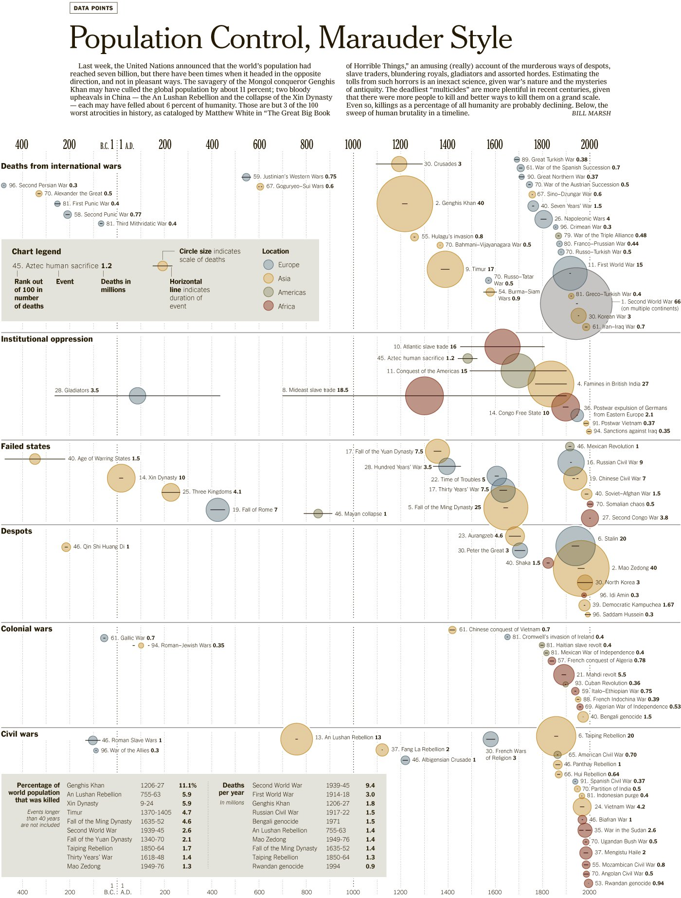
Our World in Data. (2018a). Average years of schooling (United States) [Web Page]. Our World in Data. https://ourworldindata.org/grapher/mean-years-of-schooling-long-run 

Our World in Data. (2018b). Urban and rural populations in the United States [Web Page]. Our World in Data. https://ourworldindata.org/grapher/urban-and-rural-populations-in-the-united-states 

Our World in Data. (2019a). Life expectancy, 1880 to 2019 (United States) [Web Page]. Our World in Data. https://ourworldindata.org/grapher/life-expectancy 

Our World in Data. (2019b). Population, 1800 to 2021 (Europe, United States) [Web Page]. Our World in Data. https://ourworldindata.org/grapher/population-since-1800 

Our World in Data. (2019c). Population, 1930 to 2015 (United States) [Web Page]. Our World in Data. https://ourworldindata.org/grapher/population-since-1800 

Our World in Data. (2020a). Annual working hours per worker (United States) [Web Page]. Our World in Data. https://ourworldindata.org/grapher/annual-working-hours-per-worker 

Our World in Data. (2020b). GDP per capita, 1650 to 2018 (United States) [Web Page]. Our World in Data. https://ourworldindata.org/grapher/gdp-per-capita-maddison-2020?country=~USA 

Pelteret, D. A. E. (2001). Slavery in early medieval England: From the reign of Alfred until the twelfth century. Boydell Press.

Peplow, M. (2006). Special Report: Counting the dead. Nature, 440(7087), 982–983. https://doi.org/10.1038/440982a 

Perri, A. R., Mitchell, K. J., Mouton, A., Álvarez-Carretero, S., Hulme-Beaman, A., Haile, J., Jamieson, A., Meachen, J., Lin, A. T., Schubert, B. W., Ameen, C., Antipina, E. E., Bover, P., Brace, S., Carmagnini, A., Carøe, C., Samaniego Castruita, J. A., Chatters, J. C., Dobney, K., … Frantz, L. A. F. (2021). Dire wolves were the last of an ancient New World canid lineage. Nature, 591(7848), 87–91. https://doi.org/10.1038/s41586-020-03082-x 

Peter G. Peterson Foundation. (2021, August 2). Budget Basics: National Defense [Web Page]. Peter G. Peterson Foundation. https://www.pgpf.org/budget-basics/budget-explainer-national-defense 

Philpot, R. (2018, August 5). How Britain’s Nazi-loving press baron made the case for Hitler. The Times of Israel. https://www.timesofisrael.com/how-britains-nazi-loving-press-baron-made-the-case-for-hitler/ 

Pines, Y. (2018). Legalism in Chinese Philosophy. In E. N. Zalta (Ed.), Stanford Encyclopedia of Philosophy (Winter 2018). Metaphysics Research Lab, Stanford University. https://plato.stanford.edu/archives/win2018/entries/chinese-legalism/ 

Pines, Y. (2021). 15. The Warring States Period: Historical Background. In E. Childs-Johnson (Ed.), The Oxford Handbook of Early China (pp. 581–594). Oxford University Press. https://doi.org/10.1093/oxfordhb/9780199328369.013.26 

Pollock, S. (2019). 22. Differentiation and Classification in Fourth- and Third-Millennium BC Societies. In N. Crüsemann, T. F. Potts, Vorderasiatisches Museum (Berlin, Germany), & Reiss-Engelhorn-Museen (Eds.), Uruk: First city of the ancient world (pp. 129–135). The J. Paul Getty Museum.

Popp, M., Schmidt, H., & Marotzke, J. (2016). Transition to a Moist Greenhouse with CO2 and solar forcing. Nature Communications, 7(1), 10627. https://doi.org/10.1038/ncomms10627 

Posth, C., Renaud, G., Mittnik, A., Drucker, D. G., Rougier, H., Cupillard, C., Valentin, F., Thevenet, C., Furtwängler, A., Wißing, C., Francken, M., Malina, M., Bolus, M., Lari, M., Gigli, E., Capecchi, G., Crevecoeur, I., Beauval, C., Flas, D., … Krause, J. (2016). Pleistocene Mitochondrial Genomes Suggest a Single Major Dispersal of Non-Africans and a Late Glacial Population Turnover in Europe. Current Biology, 26(6), 827–833. https://doi.org/10.1016/j.cub.2016.01.037 

Proença, V., & Pereira, H. M. (2013). Comparing Extinction Rates: Past, Present, and Future. In Encyclopedia of Biodiversity (pp. 167–176). Elsevier. https://doi.org/10.1016/B978-0-12-384719-5.00411-1 

Pugh, M. (2006). ‘Hurrah for the blackshirts!’: Fascists and fascism in Britain between the wars. Pimlico.

Qvist, S. A., & Brook, B. W. (2015). Potential for Worldwide Displacement of Fossil-Fuel Electricity by Nuclear Energy in Three Decades Based on Extrapolation of Regional Deployment Data. PLOS ONE, 10(5), e0124074. https://doi.org/10.1371/journal.pone.0124074 

Ramachandran, D., & Amir, E. (2007). Bayesian Inverse Reinforcement Learning. Proceedings of the 20th International Joint Conference on Artificial Intelligence, 2586–2591. https://www.aaai.org/Papers/IJCAI/2007/IJCAI07-416.pdf 

Ravichandar, H., Polydoros, A. S., Chernova, S., & Billard, A. (2020). Recent Advances in Robot Learning from Demonstration. Annual Review of Control, Robotics, and Autonomous Systems, 3(1), 297–330. https://doi.org/10.1146/annurev-control-100819-063206 

Razzell, P., & Spence, C. (2007). The History of Infant, Child and Adult Mortality in London, 1550–1850. The London Journal, 32(3), 271–292. https://doi.org/10.1179/174963207X227578 

Ridder-Symoens, H. de, & Frijhoff, W. (Eds.). (1996). Patterns. In Universities in early modern Europe, 1500-1800. Cambridge University Press.

Ritchie, H. (2020a). What are the safest and cleanest sources of energy? [Web Page]. Our World in Data. https://ourworldindata.org/safest-sources-of-energy 

Ritchie, H. (2020b). What was the death toll from Chernobyl and Fukushima? [Web Page]. Our World in Data. https://ourworldindata.org/what-was-the-death-toll-from-chernobyl-and-fukushima 

Rito, T., Vieira, D., Silva, M., Conde-Sousa, E., Pereira, L., Mellars, P., Richards, M. B., & Soares, P. (2019). A dispersal of Homo sapiens from southern to eastern Africa immediately preceded the out-of-Africa migration. Scientific Reports, 9(1), 4728. https://doi.org/10.1038/s41598-019-41176-3 

Roser, M., & Nagdy, M. (2013, August 6). Nuclear Weapons [Web Page]. Our World in Data. https://ourworldindata.org/nuclear-weapons 

Roser, M., Ritchie, H., & Ortiz-Ospina, E. (2019). World Population Growth [Web Page]. Our World in Data. https://ourworldindata.org/world-population-growth 

Sadao, N. (1986). Chapter 10: The economic and social history of Former Han. In D. Twitchett & M. Loewe (Eds.), The Cambridge History of China (1st ed., Vol. 1, pp. 545–607). Cambridge University Press. https://doi.org/10.1017/CHOL9780521243278.012 

Schaal, S. (1996). Learning from Demonstration. Proceedings of the 9th International Conference on Neural Information Processing Systems, 1040–1046. https://dl.acm.org/doi/10.5555/2998981.2999127 

Scheidel, W. (2007). Demography. In W. Scheidel, I. Morris, & R. P. Saller (Eds.), The Cambridge Economic History of the Greco-Roman World (1st ed., pp. 38–86). Cambridge University Press. https://doi.org/10.1017/CHOL9780521780537.004 

Scheidel, W. (2021). The Scale of Empire: Territory, Population, Distribution. In P. F. Bang, C. A. Bayly, & W. Scheidel (Eds.), The Oxford World History of Empire: Volume One: The Imperial Experience (1st ed., pp. 91–110). Oxford University Press. https://doi.org/10.1093/oso/9780199772360.003.0003 

Schneider, T., Kaul, C. M., & Pressel, K. G. (2019). Possible climate transitions from breakup of stratocumulus decks under greenhouse warming. Nature Geoscience, 12(3), 163–167. https://doi.org/10.1038/s41561-019-0310-1 

Schroder, K.-P., & Connon Smith, R. (2008). Distant future of the Sun and Earth revisited. Monthly Notices of the Royal Astronomical Society, 386(1), 155–163. https://doi.org/10.1111/j.1365-2966.2008.13022.x 

Schultz, B. (2021). Henry Sidgwick. In E. N. Zalta (Ed.), Stanford Encyclopedia of Philosophy (Winter 2021). Metaphysics Research Lab, Stanford University. https://plato.stanford.edu/archives/win2021/entries/sidgwick/ 

Selden, M., & Selden, K. (Eds.). (2015). The atomic bomb: Voices from Hiroshima and Nagasaki. Routledge.

Sepulveda, N. A., Jenkins, J. D., de Sisternes, F. J., & Lester, R. K. (2018). The Role of Firm Low-Carbon Electricity Resources in Deep Decarbonization of Power Generation. Joule, 2(11), 2403–2420. https://doi.org/10.1016/j.joule.2018.08.006 

Shakespeare, W. (2002). The Oxford Shakespeare: The Complete Sonnets and Poems (C. Burrow, Ed.). Oxford University Press. https://doi.org/10.1093/actrade/9780198184317.book.1 

Sherwood, S., Webb, M. J., Annan, J. D., Armour, K. C., Forster, P. M., Hargreaves, J. C., Hegerl, G., Klein, S. A., Marvel, K. D., Rohling, E. J., Watanabe, M., Andrews, T., Braconnot, P., Bretherton, C. S., Foster, G. L., Hausfather, Z., Heydt, A. S., Knutti, R., Mauritsen, T., … Zelinka, M. D. (2020). An Assessment of Earth’s Climate Sensitivity Using Multiple Lines of Evidence. Reviews of Geophysics, 58(4). https://doi.org/10.1029/2019RG000678 

Sider Jost, J. (2015). Prose Immortality, 1711-1819. University of Virginia Press.

Sidgwick, H. (1907). The Methods of Ethics (7th ed.). Macmillan & Co. https://www.gutenberg.org/ebooks/46743 

Silverstein Properties. (n.d.). Office Buildings—Skyscrapers || World Trade Center [Web Page]. World Trade Center. Retrieved 27 June 2022, from https://www.wtc.com/about/buildings/1-world-trade-center 

Šimčikas, S. (n.d.). Estimates of global captive vertebrate numbers [Blog]. Effective Altruism Forum. Retrieved 22 November 2021, from https://forum.effectivealtruism.org/posts/pT7AYJdaRp6ZdYfny/estimates-of-global-captive-vertebrate-numbers 

Singh, S. (2000). The code book: The science of secrecy from ancient Egypt to quantum cryptography. Anchor Books.

Siri Team. (2017, October). Hey Siri: An On-device DNN-powered Voice Trigger for Apple’s Personal Assistant [Web Page]. Apple Machine Learning Research. https://machinelearning.apple.com/research/hey-siri 

Smart, J. J. C. (1973). An outline of a system of utilitarian ethics. In B. Williams (Ed.), Utilitarianism: For and Against. Cambridge University Press. https://doi.org/10.1017/CBO9780511840852.001 

Sperling, S. (2005). Chapter 30: Monotheism and Ancient Israelite Religion. In D. Snell (Ed.), A companion to the Ancient Near East (1st ed., pp. 408–420). Blackwell Publishing.

Strope, B., & Kurzweil, R. (2017, May 17). Efficient Smart Reply, now for Gmail [Blog]. Google AI Blog. http://ai.googleblog.com/2017/05/efficient-smart-reply-now-for-gmail.html 

Thucydides. (1919). History of the Peloponnesian War (C. F. Smith, Trans.). Harvard University Press. https://doi.org/10.4159/DLCL.thucydides-history_peloponnesian_war.1919 (Original work published ca. 425 B.C.E.)

Torabi, F., Warnell, G., & Stone, P. (2018). Behavioral Cloning from Observation. ArXiv:1805.01954 [Cs]. http://arxiv.org/abs/1805.01954 

Trinity Church. (2017, June 23). The Tallest Building in New York City [Web Page]. Trinity Church Wall Street. https://trinitywallstreet.org/stories-news/tallest-building-new-york-city 

Turnbull, S. (2010). The Mongol Invasions of Japan, 1274 and 1281. Osprey Publishing.

US Congressional Budget Office. (2019). Projected Costs of U.S. Nuclear Forces, 2019 to 2028 [Report]. US Congressional Budget Office. https://www.cbo.gov/publication/54914 

US Strategic Bombing Survey. (1946). The Effects of the Atomic Bombs on Hiroshima and Nagasaki [Report]. National Archives, US Government Printing Office. https://www.trumanlibrary.gov/library/research-files/united-states-strategic-bombing-survey-effects-atomic-bombs-hiroshima-and?documentid=NA&pagenumber=1 

USDA. (2017). 2017 Census of Agriculture—Volume 1, Chapter 1: U.S. National Level Data [Dataset]. US Department of Agriculture, National Agricultural Statistics Service. https://www.nass.usda.gov/Publications/AgCensus/2017/Full_Report/Volume_1,_Chapter_1_US/ 

Vollset, S. E., Goren, E., Yuan, C.-W., Cao, J., Smith, A. E., Hsiao, T., Bisignano, C., Azhar, G. S., Castro, E., Chalek, J., Dolgert, A. J., Frank, T., Fukutaki, K., Hay, S. I., Lozano, R., Mokdad, A. H., Nandakumar, V., Pierce, M., Pletcher, M., … Murray, C. J. L. (2020). Fertility, mortality, migration, and population scenarios for 195 countries and territories from 2017 to 2100: A forecasting analysis for the Global Burden of Disease Study. The Lancet, 396(10258), 1285–1306. https://doi.org/10.1016/S0140-6736(20)30677-2 

Wainewright, W. (2017). Reporting on Hitler: Rothay Reynolds and the British press in Nazi Germany. Biteback Publishing. http://www.myilibrary.com?id=989168 

Walker, B. L. (2015). Chronology. In A Concise History of Japan (pp. xix–xxviii). Cambridge University Press. https://doi.org/10.1017/CBO9780511783043.020 

Way, R., Ives, M. C., Mealy, P., & Farmer, J. D. (2021). Empirically grounded technology forecasts and the energy transition [Working Paper No. 2021-01]. Institute for New Economic Thinking, University of Oxford. https://www.inet.ox.ac.uk/files/energy_transition_paper-INET-working-paper.pdf 

Webster, I. (2021, December 9). $4,520 in 1790 → 2021 | Inflation Calculator [Web Page]. Official Inflation Data, Alioth Finance. https://www.officialdata.org/us/inflation/1790?amount=4520 

Webster, R. (1911). Franklin, Benjamin. In Encyclopædia Britannica: Vol. Volume 11. Wikisource. https://en.wikisource.org/wiki/1911_Encyclop%C3%A6dia_Britannica/Franklin,_Benjamin 

White, M. (2011). The great big book of horrible things: The definitive chronicle of history’s 100 worst atrocities (1st ed.). W.W. Norton.

White, M. (2012). Twentieth Century Atlas—Historical Body Count [Web Page]. Necrometrics. http://necrometrics.com/pre1700a.htm#Mongol 

Williams, J. G., & Boggs, D. H. (2016). Secular tidal changes in lunar orbit and Earth rotation. Celestial Mechanics and Dynamical Astronomy, 126(1–3), 89–129. https://doi.org/10.1007/s10569-016-9702-3 

Winter, D. (n.d.-a). Different types of PONG systems [Web Page]. PONG-Story. Retrieved 4 December 2021, from https://www.pong-story.com/types.htm 

Winter, D. (n.d.-b). Pong-Story: Atari home PONG systems [Webpage]. PONG-Story. Retrieved 26 June 2022, from https://www.pong-story.com/atpong2.htm 

World Bank. (2021). Population density (people per sq. Km of land area)—Netherlands [Dataset]. World Bank. https://data.worldbank.org/indicator/EN.POP.DNST?locations=NL 

World Nuclear Association. (2020). World Nuclear Performance Report 2020 [Report No. 2020/008]. World Nuclear Association. https://www.world-nuclear.org/getmedia/3418bf4a-5891-4ba1-b6c2-d83d8907264d/performance-report-2020-v1.pdf.aspx 

Wu, Y. (2018, May 16). Smart Compose: Using Neural Networks to Help Write Emails [Blog]. Google AI Blog. http://ai.googleblog.com/2018/05/smart-compose-using-neural-networks-to.html 

Wyatt, D. (2009). Slaves and Warriors in Medieval Britain and Ireland, 800 -1200. Brill. https://doi.org/10.1163/ej.9789004175334.i-460 

Wyatt, D. (2021). Slavery in Northern Europe (Scandinavia and Iceland) and the British Isles, 500–1420. In C. Perry, D. Eltis, S. L. Engerman, & D. Richardson (Eds.), The Cambridge World History of Slavery (1st ed., Vol. 2, pp. 482–507). Cambridge University Press. https://doi.org/10.1017/9781139024723.020 

Wyndham, A. (2021, September 15). Inside DeepL: The World’s Fastest-Growing, Most Secretive Machine Translation Company [Web Page]. Slator. https://slator.com/inside-deepl-the-worlds-fastest-growing-most-secretive-machine-translation-company/ 

Yoko, O. (2015). Residues of squalor. In M. Selden & K. Selden (Eds. & Trans.), The atomic bomb: Voices from Hiroshima and Nagasaki (pp. 55–85). Routledge.

Young, S. N. R., Sack, L., Sporck-Koehler, M. J., & Lundgren, M. R. (2020). Why is C4 photosynthesis so rare in trees? Journal of Experimental Botany, 71(16), 4629–4638. https://doi.org/10.1093/jxb/eraa234 

Ziebart, B. D., Maas, A., Bagnell, J. A., & Dey, A. K. (2008). Maximum Entropy Inverse Reinforcement Learning. Proceedings of the 23rd AAAI Conference on Artificial Intelligence, 1433–1438.